Classification of brain tumor type and grade using mri texture and shape in a machine learning scheme

Magnetic Resonance in Medicine 62:1609 –1618 (2009) Classification of Brain Tumor Type and Grade Using MRI
Texture and Shape in a Machine Learning Scheme
Evangelia I. Zacharaki,1,2* Sumei Wang,1 Sanjeev Chawla,1 Dong Soo Yoo,1,3Ronald Wolf,1 Elias R. Melhem,1 and Christos Davatzikos1 The objective of this study is to investigate the use of pattern
lowing surgical biopsy or resection, but this also has lim- classification methods for distinguishing different types of brain
itations, including sampling error and variability in tumors, such as primary gliomas from metastases, and also for
grading of gliomas. The availability of an automated computer
The objective of this study is to provide an automated analysis tool that is more objective than human readers can
tool that may assist in the imaging evaluation of brain potentially lead to more reliable and reproducible brain tumor
neoplasms by determining the glioma grade and differen- diagnostic procedures. A computer-assisted classification
method combining conventional MRI and perfusion MRI is de-
tiating between different tissue types, such as primary veloped and used for differential diagnosis. The proposed
neoplasms (gliomas) from secondary neoplasms (metasta- scheme consists of several steps including region-of-interest
ses). These issues are of critical clinical importance in definition, feature extraction, feature selection, and classifica-
making decisions regarding initial and evolving treatment tion. The extracted features include tumor shape and intensity
strategies, and conventional MR imaging is often not ade- characteristics, as well as rotation invariant texture features.
quate in providing answers (1,5). Automated tools, if Feature subset selection is performed using support vector
proven accurate, can ultimately be applied to (i) provide machines with recursive feature elimination. The method was
more reliable differentiation, especially when the neo- applied on a population of 102 brain tumors histologically diag-
plasm is heterogeneous and therefore cannot be ade- nosed as metastasis (24), meningiomas (4), gliomas World
quately sampled by localized needle biopsy; (ii) avoid Health Organization grade II (22), gliomas World Health Orga-
nization grade III (18), and glioblastomas (34). The binary sup-
invasive procedures such as biopsy, especially in cases port vector machine classification accuracy, sensitivity, and
where the risks outweigh the benefits; and (iii) expedite or specificity, assessed by leave-one-out cross-validation, were,
anticipate the diagnosis (histologic examination is usually respectively, 85%, 87%, and 79% for discrimination of metas-
time consuming).
tases from gliomas and 88%, 85%, and 96% for discrimination
Toward a similar goal, researchers used conventional of high-grade (grades III and IV) from low-grade (grade II) neo-
MR imaging and echo-planar relative cerebral blood vol- plasms. Multiclass classification was also performed via a one-
ume (rCBV) maps calculated from perfusion imaging to vs-all voting scheme.
Magn Reson Med 62:1609 –1618, 2009.
differentiate between high-grade and low-grade neoplasms 2009 Wiley-Liss, Inc.
(6) or assessed the contribution of MR perfusion alone in Key words: brain tumor; MRI; classification; SVM; feature se-
differentiating certain tumor types (7,8). Many studies lection; texture; tumor grade
have used MR spectroscopy for brain tumor classification Clinical decisions regarding the treatment of brain neo- (9-11). Specifically, spectroscopic and conventional MR plasms rely, in part, on MRI at various stages of the treat- imaging was used in Wang et al. (9) to differentiate benign ment process. Radiologic diagnosis is based on the mul- from malignant brain neoplasms, applying a decision tree tiparametric imaging profile (CT, conventional MRI, ad- algorithm, whereas spectroscopic and perfusion MRI was vanced MRI). Tumor characterization is difficult because used in Weber et al. (10) to evaluate the inherent hetero- neoplastic tissue is often heterogeneous in spatial and geneity of brain neoplasms by defining four regions of imaging profiles (1), and for some imaging techniques of- interest (ROIs) in the tumoral and peritumoral region.
ten overlaps with normal tissue (especially the infiltrating Some studies used apparent diffusion coefficient maps part) (2,3). Gliomas might show mixed characteristics; for computed from diffusion tensor imaging data to differen- example, demonstrating both low- and high-grade fea- tiate metastases from primary cerebral tumors (by measur- tures. The reference standard for characterizing brain neo- ing diffusion in peritumoral edema) (12) or combined ap- plasms is currently based on histopathologic analysis fol- parent diffusion coefficient with rCBV to differentiate tu-mefactive demyelinating lesions and primary neoplasmsfrom abscesses and lymphomas (13).
The previous studies are very useful in determining the 1Department of Radiology, University of Pennsylvania, Philadelphia, Pennsyl-vania, USA clinical significance of each MR sequence separately; how- 2Laboratory of Medical Physics, School of Medicine, University of Patras, Rio, ever, they do not investigate nonlinear relationships be- tween different variables by pattern analysis. Pattern clas- 3Department of Radiology, Dankook University Hospital, Chungchungnam- sification techniques were applied for differentiating brain neoplasms based on linear discriminant analysis (LDA) *Correspondence to: Evangelia Zacharaki, PhD, Department of Radiology,University of Pennsylvania, 3600 Market St, Philadelphia, PA 19104. E-mail (14,15), or independent component analysis (16) on spec- tral intensities. Others applied support vector machines Received 9 March 2009; revised 23 June 2009; accepted 24 June 2009.
(SVMs) on perfusion MRI (17) or combined variable selec- DOI 10.1002/mrm.22147 tion and classification using bayesian least squares SVMs Published online 26 October 2009 in Wiley InterScience (www.interscience.
wiley.com).
and relevance vector machines on microarray or spectros- 2009 Wiley-Liss, Inc.
Zacharaki et al.
copy data (18). Textural features from T1 postcontrast im- used to test the robustness and accuracy of the proposed ages were employed in (19) to discriminate between met- astatic and primary brain tumors using a probabilisticneural network with a nonlinear least squares featurestransformation method. Although these studies apply MATERIALS AND METHODS
more advanced machine learning techniques, they use a We propose a multiparametric framework for brain tumor single MR sequence and do not investigate the contribu- classification and prediction of degree of malignancy. In- tion of multiple imaging parameters. Multiparametric fea- tensity- and texture-based features are integrated via a tures are explored by nonlinear classification techniques pattern classification technique into a multiparametric im- in (20,21). Li et al. (20) classify gliomas according to their aging profile. The features are first normalized to have zero clinical grade using linear SVMs trained on a maximum of mean and unit variance. A feature selection method is then 15 descriptive features (such as amount of mass effect or used to select a small set of effective features for classifi- blood supply), which are estimated quantitatively by do- cation in order to improve the generalization ability and main experts. The definition of such features is based on the performance of the classifier.
expert knowledge and therefore is not completely auto- In this section, the clinical data and the acquisition mated and reproducible. Devos et al. (21) combine stan- protocol are first reviewed. Then, the preprocessing of the dard MR intensities with spectroscopy imaging to improve data and the ROIs for feature extraction are described, classification performance using three classification tech- followed by the definition of the features. Finally, the methods for feature selection and classification are pre- In this study, we explore the heterogeneous regions of brain tumors by combining imaging features from severalsequences and extract morphologic and texture character- istics. Our analysis requires three ROIs, which define theneoplastic and necrotic region on contrast enhanced T We examined 98 patients (52 women, 46 men; age 17-83 weighted MRI, and edematous region on fluid attenuated years) with a diagnosis of brain neoplasm (from September inversion recovery (FLAIR) image. Instead of only measur- 2006 to December 2007) who had not been treated at the ing mean values in the ROIs, we investigate if conven- time of MRI. Four patients had multiple (2), not related to tional MRI has higher potential when complicated features each other, lesions that were regarded as independent are extracted, such as rotation invariant texture features masses. All patients underwent biopsy or surgical resec- based on Gabor filtering (22). Moreover, since it has been tion of the tumor with histopathological diagnosis. The shown that contrast enhancement in conventional MRI is total of 102 brain masses were histologically diagnosed not sufficient for glioma grading or differentiating between and graded based on World Health Organization criteria as metastasis and high grade tumor, we also incorporate rCBV maps. This approach incorporates imaging data which are (or can be) acquired in a routine clinical proto- gliomas grade II (22) including astrocytomas, oligo- col, including multiparametric conventional MRI and per- and gliomatosis cerebri We apply the method for binary classification, but also gliomas grade III (18) including anaplastic astrocyto- investigate the multiclass classification problem for differ- mas and (anaplastic) oligodendrogliomas entiating between the most common brain tumors: metas- glioblastomas (GBMs) (34) including 1 giant cell GBM tasis, meningioma (usually grade I), low-grade glioma(grade II), grade III glioma, and glioblastoma (grade IV) The primary sites of cancer for patients with metastatic according to the World Health Organization system. Grade lesions were lung (14), breast (5), melanoma (3), and II and grade III gliomas include astrocytomas (anaplastic or esophagus (1). For one case, the primary tumor type could not), oligodendrogliomas, and oligoastrocytomas. The pro- not be confirmed but most likely came from breast or lung.
posed framework consists of a training step, where the The study was approved by the institutional review board classifier learns the imaging characteristics of the different and was compliant with the Health Insurance Portability tumor types, and a testing step, where the classifier recog- and Accountability Act.
nizes the tumor type in a new image. The framework is The patients were imaged using a 3.0-T MRI scanner general and, if a significant number of observations (train- system (Magnetom Trio Tim System; Siemens Medical ing samples) exist, can be applied to classify any other Systems, Erlangen, Germany), with a multichannel neoplasm and also non-neoplastic pathologies, including phased-array coil. The imaging acquisition protocol was lymphoma, abscess, and encephalitis. We differentiate be- the same for all patients and includes the following se- tween tumor types by combining multiparametric MR im- quences: axial three-dimensional T1-weighted (T1) (mag- ages into a single classification rule rather than using sin- netization prepared rapid acquisition gradient echo pulse gle modalities independently. We exploit the potential of repetition time/echo time/inversion time 1760/3.1/950, features extracted automatically from the images in order matrix size 192 ⫻ 256, pixel spacing 0.9766 ⫻ 0.9766 mm, to avoid descriptive criteria, which are rater dependent slice thickness 1 mm), sagittal three-dimensional T2- and require prior knowledge (the help of experts).
weighted (T2) (matrix size 256 ⫻ 320, pixel spacing The proposed scheme consists of four parts: ROI defini- 0.8969 ⫻ 0.8969 mm, slice thickness 0.9 mm), FLAIR tion, feature extraction, feature selection, and classifica- (pulse repetition time/echo time/inversion time 9420/141/ tion based on SVMs. Leave-one-out cross-validation is 2500, matrix size 192 ⫻ 256, pixel spacing 0.9375 ⫻ Tumor Classification Using Machine Learning 0.9375 mm, slice thickness 3 mm) and diffusion tensor Feature Description imaging. Diffusion tensor imaging was not used as part of We chose a large number of features (161) for investiga- this study but will be incorporated in the future. Axial tion, which included age, tumor shape characteristics, im- three-dimensional contrast-enhanced T1-weighted images age intensity characteristics within some of the ROIs, and (T1ce) were obtained after administration of a standard Gabor texture features, as explained next.
dose (0.1 mmol/kg) of gadodiamide with a power injector(Medrad, Idianola, PA). Also, after an initial loading doseof 3 mL gadodiamide and a 5-min delay, T Shape and Statistical Characteristics of Tumor (Evaluated in ROI1 艛 ROI2 艛 ROI3) dynamic susceptibility perfusion MRI was performed us-ing a gradient echo EPI acquisition during bolus injection Five shape features (si, i ⫽ 1, . . , 5) of the total tumor area of 12 mL gadodiamide. Twenty slices were acquired with are investigated, i.e., the tumor circularity, irregularity, pulse repetition time/echo time 2000/45 ms, matrix size rectangularity, the entropy of radial length distribution of 128 ⫻ 128, pixel spacing 1.7 ⫻ 1.7 mm, slice thickness the boundary voxels, and the surface-to-volume ratio. Also 3.0 mm. rCBV maps were generated off-line by calculating three statistical features are calculated, i.e., the ratio of the change in relaxation rate using the equation ⌬R2*(t) ⫽ enhancing (venh), necrotic (vnec), and edematous (vedm) tu- ⫺ln(S(t)/S0)/TE, where S(t) is signal intensity at time t and mor volume vs total (enhancing and nonenhancing) tumor S0 is baseline signal intensity, and then integrating under the ⌬R2*(t) curve over time points corresponding to thefirst pass of the contrast bolus.
Image Intensity Characteristics The mean (␮) and variance (var) of image intensities of T Preprocessing and Definition of ROIs T1ce, T2 are calculated in the central and marginal area of The images are preprocessed following a number of steps, ROI1, ROI2 and ROI3. For FLAIR images, the same inten- including noise reduction, bias-field correction, and rigid sity characteristics are extracted from ROI4. For the rCBV intrasubject registration using the FSL library of analysis maps, since hyperintense areas are indicative but not spe- tools (23). The coregistration of all sequences (T1, T1ce, T2, cific to tumor, we first mask out areas that appear hypoin- FLAIR, rCBV) is required in order to extract features from tense in FLAIR and then calculate the mean and variance the ROIs and is performed with the rigid registration algo- of rCBV in the central and marginal region of ROI1, ROI2, rithm FLIRT (24) from FSL. The intensity levels are made and ROI4. More analytically, the voxels with low intensity comparable across subjects by histogram matching. For on the FLAIR image, such as ventricles or peripheral ves- this purpose skull stripping is first performed using brain sels in the cortical sulci, are excluded from the analysis of extraction tool (BET) (25) to generate a brain tissue mask the rCBV maps because they may represent normal vascu- from the T1 image, which is then used to extract the brain lature that may be indistinguishable from abnormal neo- region from all other coregistered sequences. A linear vascularity due to neoplastic infiltration. All intensity- transformation of the intensities (translation and scaling) related features sum up to 52 features in total. These fea- is applied in order to minimize the L 2-norm of the histo- tures are denoted as ␮C I兲, varC I兲, when measured in the gram difference between each subject and a template im- central area and ␮R 共 m I兲, varm I兲, when measured in the mar- age. Histogram matching is not applied to the rCBV maps, ginal area, where R 僆 {1, . . , 4} for ROI1 to ROI4, and I 僆 calculated from the perfusion sequence.
{T1, T1ce, T2, FLAIR, rCBV}.
The features were extracted from ROIs manually traced by two expert neuroradiologists. A maximum of four ROIs Gabor Texture The voxel-wise texture features of image I(x,y,z) are ex- ROI1 (neoplastic, enhancing), ROI2 (neoplastic, non- tracted at each tomographic slice of the three-dimensional enhancing): includes all non-necrotic enhancing neo- ROI by convoluting with 2D Gabor filters (26,27) and av- plastic tissue, or, if the lesion did not show enhance- eraging inside the ROI. The 2D Gabor filters are mathemat- ment, the whole non-necrotic T1-hypointense neo- ically described at location (x,y) as plastic tissue, avoiding peritumoral edema by tracingthe FLAIR image.
␪ ⫹ ␥2y␪ ROI3 (necrotic): this ROI is delineated only in cases g␭,␪,␴,␺共x,y兲 ⫽ exp冉 ⫺ ␭ x␪ ⫹ ␺冊 including necrotic tumor tissue by tracing the coreg-istered T1ce, T1, T2, and FLAIR images and by exclud- ing hemorrhage.
ROI4 (edematous): FLAIR and T2 images are used to depict the peritumoral edema (possibly including ␪ ⫽ xcos共␪兲 ⫹ ysin共␪兲 and y␪ ⫽ ⫺ xsin共␪兲 ⫹ ycos共␪兲 neoplastic infiltration), drawing the ROI surroundingthe high signal intensity seen on these sequences.
and ␭ ⫽ 1/f is the wavelength, ␪ the orientation, ␥ thespatial aspect ratio that determines the eccentricity of the It should be noted that the ROIs are drawn based on the convolution kernel and which was taken as ␥ ⫽ 1 in this signal intensity of different sequences and are not ex- study, and ␺ the phase offset that determines the symmetry pected to be highly specific to each tissue type. For exam- of the Gabor function. The standard deviation ␴ of the ple, nonenhancing neoplastic tissue and edematous tissue gaussian factor determines the neighborhood of a voxel in might overlap and be both present in ROI2 or ROI4.
which weighted summation takes place. The ratio ␴/␭

Zacharaki et al.
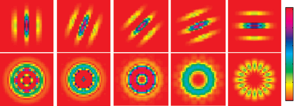
FIG. 1. Examples of filters usedto extract texture features. The1st row shows Gabor filters forsame frequency and different ori-entations, and the 2nd row, therotation-invariant filters.
determines the spatial frequency bandwidth. We used a Therefore for each bandwidth we obtain 25 rotation-in- constant ratio ␴/␭ (27), and therefore ␴ is not considered as variant texture features, gc共 I I兲, where l ⫽ 1, . . , 5 is the an independent parameter.
wavelength index and c ⫽ 1, . . , 5 is the index on fast We calculated the texture by combining the output of a Fourier transform coefficients and I 僆 { T1ce, FLAIR }. We symmetric (␺ ⫽ 0) and antisymmetric (␺ ⫽ ␲/2) Gabor used two bandwidth values (1 and 1.5) and finally ob- kernel using the L2-norm (27), as shown below: tained 100 features in total describing texture in T1ce andFLAIR for tumor classification.
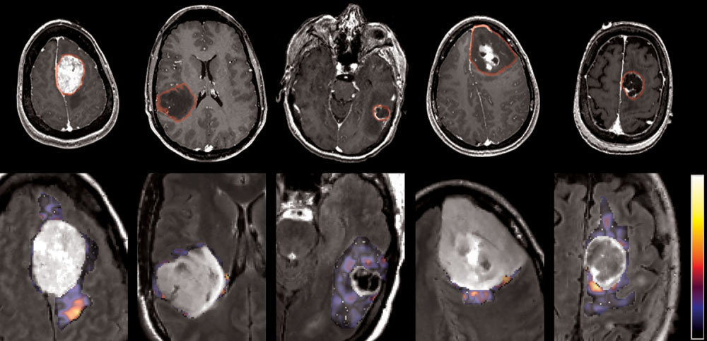
Figure 1 illustrates in the first row the Gabor filter for a single frequency across the first five (out of eight) I共x,y兲 丢 g␭ ,␪,␺⫽0 x,y兲兲2 ⫹ 共I共x,y兲 丢 g␭,␪,␺⫽␲/2 x,y兲兲2 orientations and in the 2nd row the rotation-invariant where 丢 denotes 2D linear convolution. Then, in order to filters after fast Fourier transform for the same fre- make the average Gabor features rotation invariant, for quency. Figure 2 illustrates examples of brain tumor each radial frequency f fast Fourier transform is performed types and the corresponding texture images. The first across orientation ␪ (22). Suppose we use N␪ orientations row shows one axial slice of the T1ce image with the within a period of ␲, then N␪ magnitudes of Fourier coef- tumoral region of interest (ROI1 艛 ROI2 艛 ROI3) indi- ficients can be obtained for each frequency f, but only the cated by a red line. The 2nd row shows the same slice in FLAIR image zoomed around the tumor region. As an c ⫽ N␪/2 ⫹ 1 coefficients for each frequency are example of texture, one pattern extracted from FLAIR is We extract the texture features from the T1ce in ROI1 艛 shown over the edematous area (ROI4). The illustration ROI2 艛 ROI3 and from FLAIR in ROI4. We use five wave- shows the voxelwise texture without averaging over the lengths, ␭ ⫽ 兵2冑2,4,4冑2,8,8冑2其, and N␪ ⫽ 8 orientations area of interest.
in [0, ␲] which after the fast Fourier transform produce It should be noted that texture features are affected by Nc ⫽ N␪/2 ⫹ 1 ⫽ 5 unique coefficients for each frequency.
the MRI acquisition parameters, especially the spatial res- FIG. 2. MR images of different of brain tumor types and an example of texture images extracted from the edematous area. From left to right:meningioma, glioma grade II, grade III, grade IV, and metastasis. First row: T1ce image with the tumoral region of interest. Second row:FLAIR image (zoomed in the tumor region) overlaid with one of the textural patterns (␭ ⫽ 8). This pattern is shown here as voxelwise texturefor illustration purposes and is not equivalent to our calculations. The average texture values (calculated before fast Fourier transform)(feature g54) proved to be significant in discrimination of meningiomas.
Tumor Classification Using Machine Learning olution (28). Therefore it is important to use the same graph. The remaining features (with P value ⬎ ␣) are acquisition protocol during training of the classifier and ranked by applying the t test using a bagging strategy (31).
during testing, i.e., when the classifier learns the imaging Specifically, the training set is divided in five folds and the characteristics and when the classifier recognizes a new features are ranked at each fold separately. Then the rank- case, respectively.
ings are combined to produce the total rank for each fea-ture based on forward selection.
Feature Selection Feature Subset Selection Method Based on SVM Feature selection methods can be divided into featureranking methods and feature subset selection methods SVM-based feature selection methods have been success- (29). The feature ranking methods compute a ranking score fully applied in a variety of problems. One good example for each feature according to its discriminative power and is the support vector machine recursive feature elimina- then simply select the top ranked features as final features tion (SVM-RFE) algorithm, which was initially proposed for classification. These feature selection methods are pref- for a cancer classification problem (32) and was later ex- erable for high dimensional problems due to their compu- tended by introducing SVM-based leave-one-out error tational scalability. However, the subset of features se- bound criteria in (33). The goal of SVM-RFE is to find a lected by the feature ranking methods might contain a lot subset of features that optimize the performance of the of redundant features since the ranking score is computed classifier. This algorithm determines the ranking of the independently for each feature, by completely ignoring its features based on a backward sequential selection method correlation with others. On the contrary, the feature subset that removes one feature at a time. At each time, the selection methods focus on selecting a subset of features removed feature makes the variation of SVM-based leave- that jointly have better discriminative power. In general, one-out error bound smallest, compared to removing other sophisticated subset selection methods have better classi- fication performance than feature ranking methods, but The training data set 兵 x 其 僆 ᑬn ⫻ 兵 ⫺ 1,1其 consists of their high computational cost usually limits their applica- the training patterns xk and the known class labels yk, tions to the high dimensional problems. Since combinato- where k ⫽ 1, . . , NS (NS ⫽ N1 ⫹ N2 is the total number of rial search of the optimal combination of features would be training samples belonging to both classes). We apply the computationally prohibitive, we combine the advantages zero-order method for identifying the variable that pro- of both the feature ranking method and the feature subset duces the smallest value of the ranking criterion when selection method. Specifically, we first reduce the number removed, and use the weight magnitude 储w储2 as ranking of features by eliminating the less relevant features using a criterion, defined as forward selection method based on a ranking criterion andthen apply backward feature elimination using a feature subset selection method, as explained next.
where K(i) is the Gram matrix of the training data (see Eq. 2) We use a simple ranking-based feature selection criterion, when the variable i is removed and a共i兲 is the correspond- a two-tailed t test, which measures the significance of a ing solution of the SVM classifier.
difference of means between two distributions (30), andtherefore evaluates the discriminative power of each indi- Constrained LDA vidual feature in separating two classes. If the features areassumed to come from normal distributions with un- For the purpose of comparison of the previously described known but equal variances, the t statistic is defined as: feature selection algorithm with a commonly used dimen-sionality reduction method, such as LDA, we also investi- gated the performance of the constrained LDA algorithm t ⫽ 冑共 for feature selection (34). Constrained LDA maximizes the 1兲v2冉 1 1 discriminant capability between classes without trans- forming the original features, as done by traditional LDAor principal component analysis. This is important be- where x៮1, v1 and x៮2, v2 are the sample mean and sample cause it allows preservation of the physical meaning of the variance of a particular feature in 1st and 2nd class, re- input variables and assessment of the contribution of each spectively. N1 and N2 are the number of samples in each original variable in classification.
Since the correlation among features has been com- Calculating Total Rank by Combination pletely ignored in this feature ranking method, redundantfeatures are inevitably selected, which ultimately affects Classification is performed by following a leave-one-out the classification results. Therefore, we use this feature strategy on the training samples. For each leave-one-out ranking method to select the more discriminative features, experiment, feature ranking is performed using data only e.g., by applying a cutoff ratio (P value ⬍ ⫽ ␣, where ␣ ⫽ from the training samples. The feature selection method is 0.1 is the significance level for rejecting the null hypoth- implemented in each training subset in order to correct for esis), and then apply the feature subset selection method the selection bias (35). It is important that cross-validation on the reduced feature space, as detailed in the next para- be external to the feature selection process in order to more Zacharaki et al.
accurately estimate the prediction error. Evidently, there is constant. The aim was to include a constant fraction of the no guarantee that the same subset of features will be se- training samples in a ball in feature space of size s for any lected at each leave-one-out experiment. We combine the dimensionality (number of features). The constant k was rankings of all leave-one-out experiments and report the determined such that the fraction of the training samples total rank of features (in Table 2) according to the fre- contained in the kernel is approximately 20%.
quency of a feature appearing in a specific rank. For ex- The multiclass problem was solved by constructing and ample the top-ranked feature is assumed to be the one that combining several binary classifiers into a voting scheme.
more frequently has the highest ranking score, regardless We applied majority voting from all one-vs-all binary clas- of the distribution of the scores it receives across experi- sification problems. For assessing the predictive ability of ments. In order to assess if the features are selected con- the classification scheme, we applied leave-one-out cross- sistently, we use two measures: the entropy (E) to evaluate validation. In the future, when more training data will be the certainty in ranking and the standard deviation (S) to available for each class, we will assess the generalization measure the compactness. These measures are normalized ability through 3-fold cross-validation and will further between 0 (no consistency) and 1 (same rank in all exper- optimize the classification parameters C and s for each classification problem by exhaustive search.
Classification was performed by starting with the more We applied leave-one-out external cross-validation in discriminative features and gradually adding less discrim- classifying meningioma (MEN), glioma of grades II, III, inative features, until classification performance no longer and IV (GL2, GL3, and GL4, respectively), and metasta- improved. Three pattern classification methods were in- sis (MET) by applying three different classification vestigated for comparison: LDA with Fisher's discriminant methods (LDA, kNN, nonlinear SVM) and two feature rule (36), k-nearest neighbor (k-NN) (37), and nonlinear ranking methods (t test with bagging, constrained LDA).
SVMs (33). In LDA, a transformation function is sought The results are presented in Table 1. The first column in that maximizes the ratio of between-class variance to with- Table 1 shows the tumor type to be classified. The other in-class variance. Since usually there is no transformation columns show the number of selected features (NF) giv- that provides complete separation, the goal is to find the ing the highest classification accuracy (the feature selec- transformation that minimizes the overlap of the trans- tion step was cross-validated; however, we currently formed distributions. k-NN neighbor classification is per- have no automated way of selecting the number of fea- formed based on closest training examples in the feature tures; hence, we recorded performance as a function of space. In SVMs, the original input space is mapped into a the number of features), the classification accuracy higher dimensional feature space in which an optimal (ACC), defined as the percentage of correctly classified separating hyperplane is constructed such that the dis- samples, and the area under the receiver operating char- tance from the hyperplane to the nearest data point is acteristic curve (AUC). The last row shows the corre- maximized. Due to this property, SVM classifiers tend to sponding mean values. The results show that the clas- possess good generalization ability.
sification accuracy is higher when using SVM, as ex- A critical parameter in SVM is the penalty parameter C.
pected. The number of features giving highest accuracy A larger C corresponds to assigning a higher penalty to is overall smaller when t test is used as ranking criterion misclassification. Since the data are unbalanced and the vs constrained LDA.
sample size is rather small to produce balanced classes by Subsequently, we investigated the performance of SVM subsampling the largest class, we used a weighted SVM1 using the SVM-RFE algorithm for feature selection and (38) to apply larger penalty to the class with the smaller assessed the contribution of each feature in classification.
number of samples. If the penalty parameter is not The results are shown in Table 2. The first 10 rows show weighted (equal C for both classes), there is an undesirable the classification between two single tumor types, similar bias toward the class with the large training size; thus we to Table 1, whereas the last two rows show the classifica- set the ratio of penalties for the two classes, C1 and C2, (in tion between combined types: secondary vs primary glio- each binary classification), to the inverse ratio of the train- mas (i.e., metastases vs gliomas grades II, III, IV) and low ing class sizes (38). The kernel function used in our SVM vs high grade gliomas (grade II vs III and IV). Those two classifier is gaussian radial basis function kernel. The classification problems are clinically relevant since treat- Gram matrix for two feature vectors xi,xj is defined as ment is usually adapted accordingly. Meningiomas are notincluded in the combined classification problems because 储x ⫺ 储2 they differ from the glial tumors and metastases in both origin and behavior.
Table 2 also shows the top-ranked features (thresh- where s controls the size of the gaussian kernel. We de- olded based on t statistic and ranked by the SVM-RFE fined s to be adaptive to the number of retained features algorithm for each classification task. Not all selected (NF), using the equation s ⫽ k 䡠 N 䡠 log共NF , where k is a features are shown in the third column, but only theoverall top ranked calculated by combining all leave-one-out results. The notation used for these features is described analytically in the Feature Description sec- Chang C-C, Lin C-J. LIBSVM: a library for support vector machines, 2001.
Software available at http://www.csie.ntu.edu.tw/⬃cjlin/libsvm.
tion. The subsequent columns show the sensitivity, Tumor Classification Using Machine Learning Table 1Binary Classification Accuracy (Acc) and AUC Obtained by Leave-One-Out Cross-Validation Using Different Classifiers (LDA, k-NN,SVM) and Feature Ranking Methods (t Test With Bagging or CLDA) k-NN (k ⫽ 3) specificity, accuracy, and area under the receiver oper- be a relevant pattern. It is interesting to note that usually ating characteristic values, respectively.
the large wavelengths (␭ ⫽ 8 or 8冑2) appear as part of The results of Table 2 show that perfusion is an impor- the selected patterns.
tant MR imaging technique for most classification tasks.
For most binary classification pairs, the number of fea- The enhancing portion in T1ce appears as significant pa- tures selected with SVM-RFE giving the highest classifica- rameter in the distinction of meningioma from gliomas of tion accuracy is relatively small, which means that the all grades; specifically in the case of glioblastoma, the chance of overfitting is reduced and the generalization enhancing portion in T1ce is selected as a single feature ability improved. The feature reduction is an important and achieves 97.4% accuracy. A combination of multipa- advantage of SVM-RFE over the simple t test. Although the rametric features, including T2 and T1 precontrast imaging accuracy over all classification tasks is on average almost characteristics, is used for classifying primary glioma vs the same when applying SVM-RFE as a second step after t metastasis (with accuracy 84.7%) and low- vs high-grade test, the average number of selected features over all clas- glioma (with accuracy 87.8%). Gabor texture seems also to sification tasks is overall reduced by 33% (N Table 2Binary Classification Results Obtained by Leave-One-Out Cross-Validation Using SVM for Classification and SVM-RFE for FeatureSelection Overall top-ranked features (maximum eight features are shown) enh, varm(rCBV), ␮c(T1), s3, ␮m(T2), 5(FLAIR), venh, vnec, ␮c(T1) Zacharaki et al.
Table 3Multiclass Confusion Matrix Obtained With One-Versus-All VotingScheme Using SVM Classifiers With RFE Prediction, NF ⫽ 18 (out of 50) and low- from high-grade glioma is high, as illustrated inFig. 4.
FIG. 3. Classification accuracy (with SVM-RFE) vs number of re-tained features for classification of metastasis vs gliomas grade II, Consistency in Feature Selection During Cross-Validation III, or IV (1st row) and glioma grading (2nd row).
In order to assess if the same features are selected asdiscriminant features for each leave-one-out experiment,we calculated the normalized entropy (E) and standard case of t test and N deviation (S) of the ranking scores for each feature. Aver- 20 in the case of SVM-RFE). Figure 3 and Fig. 4 (1st row) show the classification accuracy with aging of E and S across all selected features showed that increasing number of retained features. The plots illustrate the highest consistency was observed when distinguishing that the fluctuations of accuracy around the optimal num- meningioma from GBM (E៮ ⫽ 0.95, S៮ ⫽ 0.99, NF ⫽ 1), as ber of features are small and the method is not very sen- well as from gliomas grade II (E៮ ⫽ 0.82, S៮ ⫽ 0.92, NF ⫽ 9) sitive to the exact number of selected features, except in and metastasis (E៮ ⫽ 0.71, S៮ ⫽ 0.92, NF ⫽ 6).
the case of metastasis vs GBM, where the plateau is quitenarrow. The feature selection method in general elimi- nates the redundant features, reduces the noise, and builds For the multiclass problem, one-vs-all SVM classification groupings that are both robust and accurate.
and majority voting are applied. For each one-vs-all clas- Accuracy is relatively high for all classification pairs sification task, feature selection is performed using SVM- except for grade II vs grade III glioma. These two types of RFE. Since in the multiclass problem the number of clas- tumor have common characteristics due to the mixed his- sifications to be performed is large, feature selection with tology and are difficult to differentiate. On the other hand, RFE on the total number of features (161) is computation- the accuracy in classifying metastasis from primary glioma ally very expensive. For this reason, we excluded from theevaluation all features that were never (or only once) se-lected as significant features in all binary classificationtasks (Table 2). Accordingly, 50 features were retained andused for feature selection. The confusion matrix withleave-one-out cross-validation is shown in Table 3. Menin-giomas were not included due to their small sample sizeand small clinical value. The highest classification accu-racy is achieved for metastasis, where only two (out of 24)samples are misclassified (one as glioma grade III and oneas GBM) and for low-grade tumors, with two (out of 22)cases being misclassified (one as glioma grade III and oneas metastasis).
DISCUSSION AND CONCLUSIONS
This paper presents a classification scheme for differenti-ating adult brain tumors using conventional MRI and rCBVmaps calculated from perfusion MRI. Shape characteris-tics, statistics on image intensities, and rotation-invariantGabor texture features are extracted from the central andmarginal tumoral, edematous, and necrotic region. Thescheme is fully automated and the help of an expert is not FIG. 4. Classification accuracy (with SVM-RFE) vs number of re- required, except for tracing the ROIs. Overall, we found tained features (1st row) and receiver operating characteristic (ROC) that SVM-based classification of texture patterns is a very analysis (2nd row) for two main classification problems: metastasesvs primary gliomas (grades II, III, IV) shown in the 1st column and promising approach to developing an objective and quan- low- vs high-grade gliomas (grade II vs III and IV) shown in the 2nd titative evaluation of brain tumors. However larger data- sets need to be analyzed, which is expected to test the Tumor Classification Using Machine Learning generalization ability of this approach, but also to further The feature subset selection method shows that all MR improve its performance, as such classification systems sequences are important for classification since different perform better if trained more extensively.
features are selected for different classification tasks (Table The results of multiclass classification (Table 3) illus- 2). The rCBV maps calculated from perfusion seem to be trate that the highest classification accuracy is achieved for particularly important since parameters extracted from those are usually top ranked in most classification pairs.
whereas the classification accuracy for GBM is reduced Also, contrast-enhanced T1 is a significant sequence; the (29.4% are classified as grade III and 29.4% as metastasis).
volume of enhancement as percentage of total tumor vol- The lowest classification rate in the multiclass problem is ume (venh) is used as single feature for distinguishing be- for the grade III glioma, where the largest portion (44.4%) tween meningioma and GBM and is also part of the top- is classified as grade II and the smaller portions as GBM ranked features for other classification tasks. Texture cal- (11.1%) or metastasis (11.1%). The prediction of glioma culated on specific frequencies also contributes to tumor grade is inherently difficult since brain neoplasms are classification. Textural parameters extracted from the often heterogeneous, meaning that different histopatho- edematous area in FLAIR seem to be significant for glioma logic features (such as mitotic index) can be present grading, whereas texture in the neoplastic area in T1ce is throughout an individual neoplasm. Therefore, part of our important for distinguishing metastatic from glial tumors.
validation relies on examining the distribution of the false The features currently used for classification are ex- positives. The results of Table 3 show that most of the tracted from the imaging profile and describe shape and misclassified samples are assigned to a class of close de- texture. We have not incorporated features describing the gree of malignancy (grade). The degree of malignancy deformation of the healthy structure due to tumor growth.
starts from the less malignant tumors (such as meningio- It is known that different tumor types affect the surround- mas) and increases until the high grade gliomas and me- ing healthy region differently, and therefore studies have tastases. The failure of the method to classify grade III used the tumor mass effect as a descriptor for classifying gliomas possibly indicates that the extracted features do gliomas according to their clinical grade (20) or as an not form a separate cluster, but are rather similar to the independent predictor of survival (39). For this purpose, features of the nearby classes (grade II and grade IV). The we recently proposed an automated method for quantify- binary classification tasks, where only tumors from two ing the mass effect (40) by measuring how much the de- single types are compared, exhibit higher classification formation in the tumor origin deviates from the range accuracy (mean ⫽ 91%; standard deviation ⫽ 7.7% over observed in a normal population. We plan to incorporate all tasks). The highest accuracy is achieved when distin- the indicator of mass effect as an additional parameter in guishing grade II glioma from metastasis (97.8%), and the our classification framework in the future.
lowest, (75%) when distinguishing grade II from grade III Moreover, a limitation of this framework comes from the need for tracing ROIs, which makes the current approach Generally, the classification accuracy using the pro- semiautomatic and subject to intra- and interobserver vari- posed method is comparable or higher than in other stud- ability. However, it should be also noted that most of ies (6) not using spectroscopy or diffusion tensor imaging.
applied features are based on spatial averaging and there- The results in Devos et al. (21) using imaging intensities fore are not very sensitive to small differences in the de- from standard MR alone cannot be immediately compared lineation of ROIs. The most sensitive features are expected with ours because (i) they were based on ROIs extracted to be the ones calculated over the marginal area of the from spectroscopy imaging, which we want to avoid in ROIs. We have investigated in the past the use of conven- this study; and (ii) they reflected the number of voxels tional and advanced MR imaging for automatic segmenta- correctly classified rather than the number of subjects tion of neoplastic and healthy tissue (41). We plan in the (voxels from the same image were used as independent future to combine the two frameworks in order to automat- samples). In Georgiadis et al. (19), an SVM-based classifi- ically segment and classify brain neoplasms. The aim of cation system with radial basis function kernel achieved this study is to assess the discrimination ability of stan- 74.4% overall accuracy in discriminating primary brain dard MR imaging usually acquired in most clinical facili- tumors from metastases utilizing the external cross-valida- ties. The use of imaging intensities from standard MR tion method, whereas an artificial neural network classifier alone reaches lower performance than when combined performed better (80% accuracy). The features employed with spectroscopy (21). In the future, we plan to incorpo- in that study were solely textural features from the T1ce rate also diffusion tensor imaging and spectroscopy in our MR images. Our analysis, achieving 84.7% accuracy on the analysis for assessing the increase in classification accu- leave-one-out cross-validation error, also showed that Ga- racy. Other data based on microscopy imaging or his- bor textural features from T1ce are important for this clas- topathological examinations could also be included to in- sification task combined with statistical parameters (mean, crease accuracy in predictions. For example, nuclear fea- variance, etc.) from other imaging sequences (T2, rCBV).
tures extracted from segmented nuclei (42) or blood vessel Moreover, our results in glioma grading (low vs high patterns (43) can assist brain astrocytoma malignancy grade) are comparable with the ones reported in Li et al.
grading, and the spatial organization of tumor vessels can (20) (the accuracy in Li et al. (20) was assessed by cross- be indicative for differentiation between medulloblasto- validation not being external to the feature-selection pro- mas and supratentorial primitive neuroectodermal tumors cess). This study was based on descriptive features esti- (PNETs) (44). Voxel-wise histopathological parameters mated by domain experts, whereas we applied features that reflect proliferation and protein synthesis or PET im- extracted in a semiautomatic way.
aging could also be used, if available, in order to extend Zacharaki et al.
the current framework to output spatial maps of malig- 20. Li G, Yang J, Ye C, Geng D. Degree prediction of malignancy in brain nancy (instead of a single grade), providing more reliable glioma using support vector machines. Comput Biol Med 2006;36:313– differentiation of heterogenous neoplasms.
21. Devos A, Simonetti AW, van der Graaf M, Lukas L, Suykens JA, Van- hamme L, Buydens LM, Heerschap A, Van Huffel S. The use of multi-variate MR imaging intensities vs metabolic data from MR spectro- scopic imaging for brain tumour classification. J Magn Reson 2005;173: 1. Aronen HJ, Gazit IE, Louis DN, Buchbinder BR, Pardo FS, Weisskoff RM, Harsh GR, Cosgrove GR, Halpern EF, Hochberg FH, Rosen BR.
22. Tan TN. Rotation invariant texture features and their use in automatic Cerebral blood volume maps of gliomas: comparison with tumor grade script identification. IEEE Trans PAMI 1998;20:751–756.
and histological findings. Radiology 1994;191:41–51.
23. Smith SM, Jenkinson M, Woolrich MW, Beckmann CF, Behrens TE, 2. Krabbe K, Gideon P, Wagn P, Hansen U, Thomsen C, Madsen F. MR Johansen-Berg H, Bannister PR, De Luca M, Drobnjak I, Flitney DE, diffusion imaging of human intracranial tumors. Neuroradiology 1997; Niazy RK, Saunders J, Vickers J, Zhang Y, De Stefano N, Brady JM, 39:483– 489.
Matthews PM. Advances in functional and structural MR image anal- 3. Provenzale JM, Mukundan S, Baroriak DP. Diffusion-weighted and ysis and implementation as FSL. Neuroimage 2004;23(suppl 1):S208 – perfusion MR imaging for brain tumor characterization and assessment of treatment. Radiology 2006;239:632– 649.
24. Jenkinson M, Smith SA. Global optimisation method for robust affine 4. Wolde H, Pruim J, Mastik MF, Koudstaal J, Molenaar WM. Proliferative registration of brain images. Med Image Anal 2001;5:143–156.
activity in human brain tumors: comparison of histopathology and 25. Smith SM: BET: brain extraction tool. FMRIB technical report L-[l-HC] tyrosinePET. J Nucl Med 1997;38:1369 –1374.
5. Young RJ, Knopp EA. Brain MRI: tumor evaluation. J Magn Reson 26. Daugman JG. Uncertainty relations for resolution in space, spatial Imaging 2006;24:709 –724.
frequency, and orientation optimized by two-dimensional visual corti- 6. Lev MH, Ozsunar Y, Henson JW, Rasheed AA, Barest GD, Harsh GR, cal filters. J Opt Soc Am A 1985;A2:1160 –1169.
Fitzek MM, Chiocca EA, Rabinov JD, Csavoy AN, Rosen BR, Hochberg 27. Kruizinga P, Petkov N. Non-linear operator for oriented texture. IEEE FH, Schaefer PW, Gonzalez RG. Glial tumor grading and outcome Trans Image Process 1999;8:1395–1407.
prediction using dynamic spin-echo MR susceptibility mapping com- 28. Mayerhoefer ME, Szomolanyi P, Jirak D, Materka A, Trattnig S. Effects pared with conventional contrast-enhanced MR: confounding effect of of MRI acquisition parameter variations and protocol heterogeneity on elevated rCBV of oligodendrogliomas. Am J Neuroradiol 2004;25:214 – the results of texture analysis and pattern discrimination: an applica- tion-oriented study. Med Phys 2009;36:1236 –1243.
7. Kremer S, Grand S, Remy C, Esteve F, Lefournier V, Pasquier B, Hoff- 29. Guyon I, Elisseeff A. An introduction to variable and feature selection.
mann D, Benabid AL, Le Bas JF. Cerebral blood volume mapping by MR J Machine Learn Res 2003;3:1157–1182.
imaging in the initial evaluation of brain tumors. J Neuroradiol 2002; 30. Press WH, Teukolsky SA, Vetterling WT, Flannery BP. Numerical recipes in C: the art of scientific computing. New York: Cambridge 8. Provenzale JM, Mukundan S, Baroriak DP. Diffusion-weighted and University Press; 1992. 616 p.
perfusion MR imaging for brain tumor characterization and assessment 31. Breiman L. Bagging predictors. Machine Learn 1996;24:123–140.
of treatment response. Radiology 2006;239:632– 649.
32. Guyon I, Weston J, Barnhill S, Vapnik V. Gene selection for cancer 9. Wang Q, Liacouras EK, Miranda E, Kanamala US, Megalooikonomou V.
classification using support vector machines. Machine Learn 2002;46: Classification of brain tumors using MRI and MRS. In: Proceedings of 389 – 422.
the SPIE Conference on Medical Imaging, 2007.
33. Rakotomamonjy A. Variable selection using SVM-based criteria. J Ma- 10. Weber MA, Zoubaa S, Schlieter M, Ju¨ttler E, Huttner HB, Geletneky K, chine Learn Res 2003;3:1357–1370.
Ittrich C, Lichy MP, Kroll A, Debus J, Giesel FL, Hartmann M, Essig M.
34. Zifeng C, Baowen X, Weifeng Z, Dawei J, Junling X. CLDA: feature Diagnostic performance of spectroscopic and perfusion MRI for distinc- selection for text categorization based on constrained LDA. Interna- tion of brain tumors. Neurology 2006;66:1899 –1906.
tional Conference on Semantic Computing, p 702–712.
11. Cho Y-D, Choi G-H, Lee S-P, Kim J-K. 1H-MRS metabolic patterns for 35. Ambroise C, McLachlan GJ. Selection bias in gene extraction on the distinguishing between meningiomas and other brain tumors. Magn basis of microarray gene-expression data. Proc Natl Acad Sci USA Reson Imaging 2003;21:663– 672.
12. Higano S, Yun X, Kumabe T, Watanabe M, Mugikura S, Umetsu A, Sato 36. Lachenbruch PA. Discriminant analysis. New York: Hafner Press; 1975.
A, Yamada T, Takahashi S. Malignant astrocytic tumors: clinical im- 37. Dasarathy BV, editor. Nearest neighbor (NN) norms: NN pattern clas- portance of apparent diffusion coefficient in prediction of grade and sification techniques. 1991.
prognosis. Radiology 2006;241:839 – 846.
38. Huang Y-M, Du S-X. Weighted support vector machine for classifica- 13. Al-Okaili RN, Krejza J, Woo JH, Wolf RL, O'Rourke DM, Judy KD, tion with uneven training class sizes. Proceedings of 2005 International Poptani H, Melhem ER. Intraaxial brain masses: MR imaging– based Conference on Machine Learning and Cybernetics, 2005. p 4365– 4369.
diagnostic strategy—initial experience. Radiology 2007;243:539 –550.
39. Lacroix M, Abi-Said D, Fourney DR, Gokaslan ZL, Shi W, DeMonte F, 14. Tate AR, Majo´s C, Moreno A, Howe FA, Griffiths JR, Aru´s C. Automated Lang FF, McCutcheon IE, Hassenbusch SJ, Holland E, Hess K, Michael classification of short echo time in in vivo 1H brain tumor spectra: a C, Miller D, Sawaya RA. Multivariate analysis of 416 patients with multicenter study. Magn Reson Med 2003;49:29 –36.
glioblastoma multiforme: prognosis, extent of resection, and survival.
15. Majo´s C, Julia -Sape´ M, Alonso J, Serrallonga M, Aguilera C, Acebes JJ, J Neurosurg 2001;95:190 –198.
Aru´s C, Gili J. Brain tumor classification by proton MR spectroscopy: 40. Zacharaki EI, Hogea CS, Shen D, Biros G, Davatzikos C. Non-diffeomor- comparison of diagnostic accuracy at short and long TE. Am J Neuro- phic registration of brain tumor images by simulating tissue loss and radiol 2004;25:1696 –1704.
tumor growth. Neuroimage 2009;46:762–774.
16. Huang Y, Lisboa PJG, El-Deredy W. Tumour grading from magnetic 41. Verma R, Zacharaki EI, Ou Y, Cai H, Chawla S, Wolf R, Lee S-K, resonance spectroscopy: a comparison of feature extraction with vari- Melhem ER, Davatzikos C. Multi-parametric tissue characterization of able selection. Stat Med 2003;22:147–164.
brain neoplasms and their recurrence using pattern classification of MR 17. Emblem KE, Zoellner FG, Tennoe B, Nedregaard B, Nome T, Due- images. Acad Radiol 2008;15:966 –977.
Tonnessen P, Hald JK, Scheie D, Bjornerud A. Predictive modeling in 42. Glotsos D, Tohka J, Ravazoula P, Cavouras D, Nikiforidis G. Automated glioma grading from MR perfusion images using support vector ma- diagnosis of brain tumours astrocytomas using probabilistic neural chines. Magn Reson Med 2008;60:945–952.
network clustering and support vector machines. Int J Neural Syst 18. Lu C, Devos A, Suykens JAK, Arus C, Van Huffel S. Bagging linear sparse bayesian learning models for variable selection in cancer diag- 43. Selby DM, Woodard CA, Lakshman-Henry M, Bernstein JJ. Are endo- nosis. IEEE Trans Informat Technol Med 2007;11:338 –346.
thelial cell patterns of astrocytomas indicative of grade? In Vivo 1997; 19. Georgiadis P, Cavouras D, Kalatzis I, Daskalakis A, Kagadis GC, Sifaki K, Malamas M, Nikiforidis G, Solomou E. Improving brain tumor char- 44. Goldbrunner RH, Pietsch T, Vince GH, Bernstein JJ, Wagner S, Hage- acterization on MRI by probabilistic neural networks and non-linear man H, Selby DM, Krauss J, Soerensen N, Tonn JC. Different vascular transformation of textural features. Comput Methods Programs Biomed patterns of medulloblastoma and supratentorial primitive neuroecto- 2008;89:24 –32.
dermal tumors. Int J Dev Neurosci 1999;17:593–599.

Source: http://biosignal.med.upatras.gr/ezachar/papers/MRM_TumorClassif_2009.pdf