Cao-rhms.ru

TURBULENT INVERSION AND ENTRAINMENT INTO STRATOCUMULUS TOPPED Szymon P. Malinowski1, Marta K. Kopeć1, Wojciech Kumala1, Katarzyna Nurowska1 Hermann Gerber2, DjamalKhelif3 1University of Warsaw, Faculty of Physics, Institute of Geophysics, Pasteura 7, 02-093 2Gerber Scientific Inc., Reston, VA, USA. 3Department of Mechanical & Aerospace Engineering and Earth System Science, University of California Irvine, CA, USA. structured in a following way: information of Exchange processes between stratocumulus POST and key instruments are in section 2, and free troposphere above have been data from two contrasting cases TO10 and intensively investigated in many research TO13 are described in section 3 and campaigns (see e.g. Albrecht et al. (1988), discussed in section 4.
Lenshow et. al. (1988), Stevens et al. (2003), 2. POST: PHYSICS OF STRATOCUMULUS Bretherton et al. (2004)). Despite the fact that TOP RESEARCH CAMPAIGNmarine stratocumulus is a relatively simple Physics of Stratocumulus Top (POST) was a system: almost plain-paral el, warm cloud research campaign held in the vicinity of occupying the upper part of the well mixed Monterey Bay in July and August 2008. High- boundary layer above a homogeneous flat resolution in-situ measurements with surface, understanding entrainment into the CIRPAS Twin Otter research aircraft were stratocumulus topped boundary layer (STBL) focused on a detailed study of processes is limited. Consequently, estimates of the occurring at the interface between the STBL entrainment velocity are ambiguous (e.g. and the free troposphere. The aircraft was Stevens (2002), Gerber et al. (2005), equipped to measure thermodynamics, Faloona et al. (2005), Lil y (2008)). Data from microphysics, dynamics and radiation.
in-situ measurements (e.g. Caughley et al. (1982), Nichol s (1989), Lenshow et. al. (2000), Rode and Wang (2007)) and results of numerical simulations (e.g. Moeng et.al. (2005), Yamaguchi and Randall (2008)) clearly indicate that top of the stratocumulus is located below the capping inversion and does not touch the free troposphere. In between there is so-called entrainment interface layer, EIL, of thickness varying from few meters to few tens of meters Gerber et al., (2002), Haman et al. (2007), Kurowski et.al., (2009). Data from the majority of field campaigns and numerical simulations are of too poor resolution to infer about details of this layer. 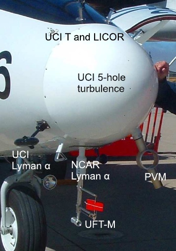In this note we present two cases of very di e ff rent structures of stratocumulus top, capping inversion and EIL, documented Figure 1. Radome of CRPAS Twin Otter research by means of very high spatial resolution aircraft with fast-response instruments used in measurements of temperature and liquid POST.
water content. Analyzed airborne data were Adopted flight strategy was aimed at collected in course of Physics of col ection of data from the cloud-top region, Stratocumulus Top (POST) research accompanied by information on fluxes in campaign performed in 2008 Gerber et al. various levels of STBL and vertical profiles of (2010, 2012). The present document is thermodynamic and dynamic parameters al owing to characterize lower atmosphere for the purpose of Large Eddy Simulations. 3. TWO CASES: TO10 AND TO13 FLIGHTSOf key interest was cloud top, sampled in 3.1. CLASSICAL CASE TO10 course of porpoises across EIL, as shown in Fig.3 of Gerber et al. (2010). In this study we Flight TO10 was performed on 2008/08/04, focus on a fine-scale measurements 17:15-22:15 UTC. It was a daytime flight collected with the UFT-M thermometer (local time was UTC -7h) in a fairly uniform Kumala et al. (2012), Particulate Volume cloud field (c.f. satel ite images in POST Monitor PVM-100 Gerber et al. (1994), and database). Typical sounding, taken in course other fast-response instruments col ocated in of TO10 (Fig.2), shows a sharp liquid water close proximity around the radome of the potential temperature θl jump (10K) in 3 aircraft (Fig.1). The finest resolution PVM thick layer above the cloud top, accompanied and UFT-M data discussed here are of by a rapid drop of water vapor mixing ratio 1000Hz sampling frequency, which and a substantial wind shear ( 4 ∼ m/s for each ∼ .5cm spatial resolution at component of wind velocity). 55m/s true airspeed (TAS) of Twin Otter. In Fig.3 records of temperature T, liquid Other fast response sensors provided 100Hz water content LWC, pressure corrected and 40Hz (55cm and 1.4m spatial resolution) altitude h, water vapor mixing ratio r and measurements of three components of fluctuations of three components of velocity turbulent velocity fluctuations and humidity. (u,v,w) in course of typical descend into the Data are freely available from the POST cloud deck are presented. Three black database maintained by by National Center vertical lines discriminate between the layers of Atmospheric Research Earth Observation of substantial y di e ff rent properties. The first one, corresponding to the left part of the plot is a free troposphere (FT) above the Preliminary analysis of col ected data inversion. Temperature, water vapor mixing performed by Gerber et al. (2010, 2012) ratio and velocity records are smooth, allowed to distinguish between "classical" fluctuations are small.
and "nonclassical" cases. Out of 17 research The first black line set at 67726s (659m flights performed in course of campaign, 6 altitude) marks the end of FT layer. After the were characterized as "classical" and 9 as marker temperature decreases, fluctuating "non-classical". In the fol owing we analyze rapidly. Velocity records show presence of a details of EIL structure in "classical" TO10 substantial wind shear and turbulence. case and "non-classical" TO13 in order to Temperature jump of 8 ∼ K is recorded in understand similarities and di e ff rences ∼13m thick layer on a horizontal distance of between the cases.
∼550m. Such temperature drop, wind shear and turbulence are common features for al porpoises in this flight, suggesting existence of a characteristic Turbulent Inversion Sub-Layer (TISL) above the cloud top. It is worth noticing, that vapor pattern not always mirrors that of T. Increased humidity spots, indicating former mixing events (detrainment), are present in FT above TISL.
2nd marker, set at 67736s (644m altitude), indicates entrance into a first blob of a cloud (LWC>0). Later aircraft penetrates through a series of cloudy and clear filaments. Inside the last ones a remarkable (amplitude 2 temperature fluctuations are present. Horizontal velocities indicate continuing wind Figure 2. Vertical profiles of potential temperatures,mixing ratios and components of shear, slightly weaker than in TISL. Turbulent horizontal wind characteristic for TO10 research velocity fluctuations are increased. flight. Cloud layer marked with a gray box. Intertwined cloudy and clear air filaments are recorded on a distance of 8 thick layer. This region is named a Cloud Top Figure 3. Temperature T, liquid water content LWC, water vapor mixing ratio q and velocity fluctuations (mean value substracted) in course of descend (h-altitude) into the stratocumulus cloud deck. Three black vertical lines mark borders between the free troposphere, the inversion, the cloud mixing layer and the cloud top. Mixing Sub-Layer (CTMSL). CTMSL together In Fig.4 three expanded segments of 1000Hz with TISL forms the Entrainment Interface LWC and T records from CTMSL are Layer, EIL.
presented in order to demonstrate character The rightmost black mark at 67751s (628m of smal -scale T and LWC fluctuations. It can altitude) indicates entrance into the cloud top be seen that local y, in cloudy filaments, layer (CTL). There are remarkable LWC approaches 0.6gm-3 , i.e. the maximum fluctuations of LWC inside CTL, but its value value across the whole cloud depth. These at 100Hz (55cm spatial resolution) record is filaments are cold, of temperature 9 everywhere above 0. Temperature characteristic for the CTL. Some cloudy fluctuations are smal , typical y of 0.2oC, in filaments with depleted LWC are warmer, of contrast to that in CTMSL where they exceed temperatures 10.2-10.6oC. Fluctuations of 2oC. Velocity fluctuations are still large, LWC in CTMSL are steeper than fluctuations especially of a vertical component.
of T. Sometimes (e.g. at 67736.8s) a shift Figure 4. Ful 5.5cm resolution (1000Hz) blow-ups of T and LWC fluctuations in the cloud mixing layer. Time corresponds to that in Fig.3. Two upper panels show 1s (55m long) segments, the bottom one shows 2s (110m long) segment. between LWC and T peaks can be noticed, Wind jump in the cloud top region is smal er most likely e e ff rent location of PVM than in TO10 case and a shear layer is and UFT sensors.
significantly deeper, its bottom correlates Vertical profiles of LWC across CTMSL and with the top of the mixed boundary layer.
CTL from 12 consecutive typical penetrations are presented in Fig.5. Each dot corresponds to LWC averaged over 1.4m long distance (40Hz data). In most subplots the maximum LWC increases linearly with height, suggesting presence of parcels lifted (almost) adiabatical y from the cloud base, (c.f. Pawlowska et.al., (2000), Gerber (1996)). Parcels with reduced LWC most often appear in CTMSL, in CTL depleted LWC is less common and indicates presence of "cloud holes" (Gerber et al. (2005), Kurowski et.al. (2009), Malinowski et al. (2012)), parcels of negative buoyancy, formed in course of mixing and evaporative Figure 6. As in Fig.2, but for TO13 flight.
cooling at the cloud top, slowly descending In Fig.7 100Hz series of T, LWC, r and across the cloud deck.
velocity fluctuations in typical penetration of the cloud top are presented. In contrast to TO10 case (c.f. Fig.4), T, r and velocity fluctuations are present in FT above EIL. Line discriminating between FT and TISL is set at 14746s (altitude of 599m), marking beginning of the sharp inversion associated with a wind shear (v velocity component only). Patterns of T and v before the marker suggest wavy engulfment of FT air into TISL.
A first blob of cloudy air (14751s, 591m height) marks beginning of CTMSL. There Figure 5. Typical profiles of LWC col ected on are increased velocity fluctuations associated porpoises in TO10 flight. Each data point with this parcel and successive cloud blobs. corresponds to 1.4m long average (40Hz data). Later, til 14772s (down to 554m altitude) T, r Four consecutive profiles are shown in each row. Successive rows are from different flight legs in and LWC vary. Except for the first cloudy order to il ustrate LWC profiles for the the whole filament, LWC in CTMSL does not exceed flight. 0.25gm-3 , which is substantial y less than the maximum LWC in cloud top region. This 3.2. NON-CLASSICAL CASE TO13 suggests that cloud filaments in this region Conditions during evening flight TO13, do not contain adiabatic parcels originating at performed 2008/08/09, 00:58-06:00 UTC the cloud base. Humidity in both cloud and were different, as il ustrated in Fig.6. While clear air filaments approaches the saturation the total jump of θ l between the middle of the mixed layer and the 1 ∼ 000m altitude is A marker discriminating between CTMSL and comparable to TO10 case ( 1 ∼ 0K), a sharp CTL is set in a point in which LWC jump inversion above the cloud top has a correlates with drop of T and r. Right to this temperature jump of no more than 4 ∼ K. θl point there are remarkable fluctuations of and total water profiles are tilted from vertical LWC and of all velocity components, but no across the upper part of the cloud. This more systematic increase of v (end of wind suggests that the cloud top is not a part of shear layer). Across the whole depth of EIL the mixed atmospheric boundary layer.
(between 599m and 554m) temperature Humidity profile in Fig.6 shows almost changes by less than 2.5K, v velocity saturated layer (or blob?) at 7 ∼ 50m height. component changes by paradoxical y, water vapor mixing ratio Figure 7. As in Fig.3, but for TO 13 flight.Figure 3. increases with height, indicating that the in Fig.6. Di e ff rences between these figures whole EIL is close to saturation.
are striking. In TO10 maximum LWC in CTL Fig.8 shows 1000Hz blow-ups of T and LWC and CTMSL in 100m thick layer at the cloud fluctuations in CTMSL. Microscale picture of top increases with height, in TO13 it cloud-clear air mixing clearly di e ff rs from that decreases or is constant. Several panels in TO10 (c.f. Fig.5). Regions of LWC<0.1g/m3 indicate that in a layer below 100-150m from accompanied by temperature fluctuations of the cloud top the maximum LWC shows ∼0.5K are common. Sharp ramps in pattern typical to that in the mixed layer: a temperature record suggest very narrow linear increase of maximum LWC with the interfaces between the filaments of various altitude. temperatures. Such ramps, common within It is worth of mentioning, that structure of both: cloudy and clear air filaments were not stratocumulus top in TO13 is not unique. It observed in TO10 case. resembles closely e.g. clod top from RF08B In Fig.9 twelve consecutive vertical profiles of case of FIRE I research campaign (c.f. Fig 6 LWC in are presented in a similar manner as in Rode and Wang (2007)).
Figure 8. As in Fig.4, but for TO 13 flight. Panels 1 and 3 show 2s (110m long) segments, in the middle panel1s (33m long) segment is presented. ff rences in thermodynamical and dynamical properties of the cloud tops between TO10 and TO13 cases were reflected in visual appearance of where g is gravity acceleration, ∆ϑl, ∆u and stratocumulus top. Observers on board ∆v are jumps of liquid water potential noticed "classic stratocumulus layer" in temperature and horizontal velocity course of TO10 flight, while in course of components across the layer of thickness of TO13 they reported "cloud tops looking like ∆z.
Vertical gradients are a e ff cted by the way data were collected. Almost horizontal flight path (typical inclination 2 degrees) and inevitable horizontal variability of temperature and wind are cause of this problem. In particular, CTMSL as seen in Figs. 3 and 6, may not appear on vertical profiles from. e.g. dropsondes. Thickness of this sublayer is just a "first guess" estimate of the amplitude of cloud top fluctuations on a horizontal distance of few km.
Figure 9. As in Fig.5, but for TO13 flight. Keeping above in mind, a simplified dynamical picture of cloud top region in both, Nature of these di e ff rences requires such di e ff rent cases, is surprisingly similar. additional analysis. Consider crude estimates Free troposphere is dynamical y stable of turbulence parameters in consecutive (Ri≈4), with the minimum values of RMSV in layers and sublayers of the cloud top region al the investigated layers. TISL, CTMSL and (Table 1), based on few penetrations in each the whole EIL are characterized by values of Ri close to the critical (which, according to di e ff rent sources varies in a range 0.2–1.0). Minimum value of Ri seems to be characteristics of TISL. Al the penetrations seen by the authors so far confirm that TISL is turbulent, despite the maximum static stability across this layer. SiA border between non-turbulent FT and turbulent TISL is Table 1. Typical properties of turbulence in always sharp, no gradual increase of velocity consecutive layers of the cloud top in TO10 and fluctuations is observed. CTL begins at the level where horizontal velocity gradient Rows: FT-free troposphere, TISL- turbulent vanishes. Similar properties of EIL, col ected inversion sublayer, CTMSL- cloud top mixing from helicopter-borne instrumented platform sublayer, CTL- cloud top layer, EIL: entrainment interfacial layer. ACTOS were reported by Katzwinkel et al., (2011). Columns: RMSV- root mean square velocity in m/s, Ri- bulk Richardson number, LC – Corrsin Estimates of Ri and RMSV across whole EIL scale, LO – Ozmidov scale. are more reliable than across the sublayers. Root mean square velocity (RMSV) Despite the uncertainties, turbulent fluctuations were calculated using low-pass properties of EIL as diagnosed from Ri are filtered velocity (10Hz cutoff frequency) in similar in both cases. This can be explained order to damp the instrumental noise. Bulk analyzing the length scales associated with Richardson number was estimated from 1 Hz the turbulence. The first one, Corrsin scale, is ∼ 0m thick layer of FT, and the a scale above which eddies are deformed by whole depths of TISL, CTMSL and EIL using the shear and can be expressed as: the fol owing formula: In the above S is velocity shear across the fraction χ<0.11 are saturated after EIL and ε is the turbulent kinetic energy completion of mixing. This means, that dissipation rate. Ozmidov length scale is a diluted cloudy parcels of χ<0.12 are likely to scale above which eddies are deformed by a be removed from CTML by negative stable stratification in EIL and is expressed buoyancy. as: In contrary, for TO13 case, mixing across inversion cannot produce negative buoyancy. High RH of entrained FT air and smal where N is Brunt-Vaisala frequency across temperature di e ff rence between FT and CTL the EIL. While we do not know ε in both cause that evaporative cooling in course cases (estimates from the power spectra of mixing is weak, which only marginal y a e velocity on short flight segments are not buoyancy (density). Additional y, mixtures of reliable), we can estimate the ratio of Corrsin as high fraction of clear air as χ<0.7 are stil and Ozmidov scales: cloudy. In consequence, most of the mixed parcels maintain diluted cloud water and remain close to the level where mixing occurred, which leads to formation of a layer The last equation shows link between the with reduced LWC below the inversion. scale ratio and Ri which can be interpreted in 5. CONCLUSIONS a fol owing way: production of turbulence by the shear and across EIL and its damping by 1. Inversion capping stratocumulus layer is the buoyancy across EIL coincides. Ri in turbulent.
range 0.3-0.5 in statically stable turbulent mixing layers is widely reported in the 2. Exchange between FT and CTL is literature (see review by Peltier and Caulfield governed by turbulent mixing across EIL. (2003)), direct numerical simulations of Thickness of EIL results from dynamic Smyth and Moum (2000) (c.f. Fig 6 therein), adaptation of thickness of the shear layer to of Brucker and Sarkar (2007) (Fig.7 therein) temperature (density) and wind jumps and of Pham and Sarkar (2010) (Fig. 2B between CTL and FT. Adaptation means therein); consequently show Ri in range 0.3- maintaining the Richardson number close to 0.5 in the stratified shear layer in agreement its critical value.
with the laboratory experiments reviewed by 2. Despite similarities in dynamics of Peltier and Caulfield (2003) and with our exchange process across EIL, existence or estimates. More interestingly, Peltier and non-existence of cloud top entrainment Caulfield (2003) discuss details of the instability leads to substantial di e mechanism which drives mixing across the Sc top structure. When thermodynamic stratified shear layer: overturning of densities conditions allow CTEI, mixed parcels which in Kelvin-Helmhols billows leading to are negatively buoyant they are removed secondary convective instability across the from CT region due to negative buoyancy. layer which determine mixing e ci ffi ency. For high RH of FT, preventing from CTEI, ff rs Sc cloud top mixing region from mixed parcels often remain cloudy and stable mixing layers reviewed in the literature buoyancy sorting prevents them from ff ct of evaporative cooling in course sinking. They remain in the cloud top region of mixing, leading to nonlinear e e ff cts in below inversion. buoyancy of mixed parcels. Relative humidity
RH of FT in TO10 case is 0.12, while in TO13 Acknowledgments:
This research was it reaches 0.92. In both cases CTL is supported by the National Science Foundation saturated containing small, typical for with the grant ATM-0735121 and by the Polish stratocumulus clouds, amounts of LWC. Ministry of Science and Higher Education with the Mixing diagram for TO10 case closely grant 186/W-POST/2008/0. We thank al resembles that from RF01 of DYCOMS II POSTers and CIRPAS for the excel ent experiment (c.f. Fig. 11 in Kurowski et.al. col aboration during the field campaign. The manuscript was written in Kavli Institute for (2009)). For dry troposphere parcels Theoretical Physics at UC Santa Barbara in containing FT fraction χ<0.12 in mixing event course of "Nature of Turbulence" program, SPM are negatively buoyant, and mixtures of FT acknowledges support from KITP. Smal scale mixing processes at the top of a marine stratocumulus - A case study, Albrecht, B.A., Randal , D.A., Nicholls, S. Q.J.R.Meteorol.Soc., 133, 213–226.
(1988), Observations of marine Katzwinkel, J., H. Siebert, and R. A. Shaw. (2011), Observation of a self-limiting, fire,Bul .Amer.Meteor.Soc., 69, 618–626.
shear-induced turbulent inversion layer Bretherton, C.S., Uttal, T., Fairal , C.W., above marine stratocumulus. Boundary- Yuter, S.E.,Wel er, R.A., Baumgardner, D., Comstock, K., Wood. R., Raga, G.B. (2004), The Epic 2001 Stratocumulus Kumala, W., Haman, K.E., Kopec, M.K., Study, Bul .Amer.Meteor.Soc., 85, 967– Malinowski, S.P. (2012), Ultrafast Thermometer UFT-M: High Resolution Brucker, K.A., Sarkar, S. (2007), Evolution of Temperature Measurements During an initially turbulent stratified shear layer, Physics of Stratocumulus Top (POST), in Phys.Fluids, 19, 1050105.
preparation to Atmos Meas.Tech.
Caughey, S. J.,Crease, B. A., Roach, W. T. Kurowski, M.J., Malinowski, S.P., Grabowski, (1982), A field study of nocturnal W.W. (2009), A numerical investigation of stratocumulus: II. Turbulence structure entrainment and transport within a and entrainment, Q.J.Roy.Meteor.Soc., stratocumulus-topped boundary layer, 108, 125–144.
Q.J.R.Meteorol.Soc., 135, 77–92.
Faloona, I., Lenschow, D.H, Campos T., Lenschow, D. H., Paluch, I.R., Brandy, A.R, Stevens, B., van Zanten, M. (2005), Pearson, R., Kawa S.R, Weaver C.J., Kay, Observations of Entrainment in Eastern J.G, Thornton D.C., Driedger A.R., (1988), Pacific Marine Stratocumulus Using Three Dynamics and Chemistry of Marine Conserved Scalars, J.Atmos.Sci., 62, Stratocumulus (DYCOMS) Experiment, Bul .Amer.Meteor.Soc., 69, 1058–1067.
Gerber, H., Arends, B.G., Ackerman, A.S. Lenschow, D.L., Zhou, M., Zeng, X., Chen, (1994), A new microphysics sensor for L., Xu, X., (2000), Measurements of fine- aircraft use, Atmos.Res., 31, 235–252.
scale structure at the top of marine Gerber, H. (1996), Microphysics of Marine stratocumulus, Boundary Layer Meteorol., Stratocumulus Clouds with Two Drizzle 97, 331–357.
Modes, J.Atmos.Sci., 53, 1649–1662.
Lilly, D. K. (1968) Models of cloud-topped Gerber , H., S.P. Malinowski, J.-L Brenguier, mixed layers under a strong inversion, and F. Burnet (2002): On the entrainment Q.J.R.Meteorol.Soc., 94, 292–309.
process in stratocumulus clouds. Proc. Lilly, D. K. (2008), Validation of a mixed-layer 11th Conf. On Cloud Physics, Ogden, UT, closure. II: Observational tests, Amer. Meteor. Soc., CD-ROM, paper Q.J.R.Meteorol.Soc., 134, 57–67.
Malinowski, S.P., Haman, K.E, Kopec M.K., Gerber, H., Frick, G., Malinowski, S.P., Kumala, W., Gerber H.E., Krueger, S.K Brenguier, J-L., Burnet, F. (2005), Holes (2010),Small scale variability of and entrainment in stratocumulus, temperature and LWC at Stratocumulus J.Atmos.Sci., 62, 443–459.
top , 13th Conference on Cloud Physics, Gerber, H., Frick, G., Malinowski, S.P., Portland, OR, 2010, American Kumala, W., Krueger, S. (2010), POST-A New Look at Stratocumulus, 13th Conference on Cloud Physics, Portland, OR, 2010, American Meteorological Moeng C-H., Stevens B., Sullivan PP. (2005), Where is the interface of the stratocumulus-topped PBL?, J. Atmos. Sci., 62, 2626–2631.
Gerber, H., Frick, G., Malinowski, S.P, Nichol s, S. (1989), The structure of Jonsson H., Khelif D., Krueger S. (2012): radiatively driven convection in Entrainment in Unbroken Stratocumulus. stratocumulus, Q.J.R.Meteorol.Soc., 115, submitted to J.Geophys. Res.
Haman, K.E., Malinowski, S.P., Kurowski, Pawlowska, H., Brenguier, J-L., Burnet, F. M.J., Gerber, H., Brenguier, J-L. (2007), (2000), Microphysical properties of stratocumulus clouds, Atmos.Res., 55, Yamaguchi, T., Randal , D.A., (2012), Cooling 15–23.
of entrained parcels in a large-eddy Peltier, W.R., Caulfield C.P. (2003), Mixing simulation. J.Atmos. Sci., 69, 1118-1136.
Efficiency in stratified shear flows.Annu.Rev.Fluid.Mech., 35, 135–167.
Pham, H.T., Sarkar, S. (2010), Transport and mixing of density in a continuously stratified shear layer.J.of.Turbulence, 11, 1–23.
Roode, S.R., Wang, Q. (2007), Do stratocumulus clouds detrain? FIRE I data revisited, Boundary-Layer Meteorol., 122, 479–491.
Smyth, W.D., Moum, J.N. (2000), Length scales of turbulence in stably stratified mixing layers, Phys.Fluids, 12, 1327–1342.
Sorbjan, Z. (2010), Gradient-based scales and similarity laws in the stable boundary layer, Q.J.R.Meteorol.Soc., 136, 1243–1254.
Stevens, B. (2002), Entrainment in stratocumulus-topped mixed layers, Q.J.R.Meteorol.Soc., 128, 2663-2690.
Stevens, B., Lenschow, D.H., Vali, G., Gerber, H., Bandy, A., Blomquist, B., Brenguier, J-L., Bretherton, C. S., Burnet, F., Campos, T., Chai, S., Faloona, I., Friesen, D., Haimov, S., Laursen, K., Lilly, D.K., Loehrer, S.M., Malinowski, S.P., Morley, B., Petters, M.D., Rogers, D.C., Russell, L., SavicJovcic, V., Snider, J.R., Straub, D., Szumowski, M.J., Takagi, H., Thornton, D.C., Tschudi, M., Twohy, C., Wetzel, M., van Zanten, M.C. (2003), Dynamics and chemistry of marine stratocumulus - Dycoms II, Bull. Amer. Meteorol.Soc., 84, 579–593.
Stevens B., Moeng C.H., Ackerman A.S., Bretherton C.S., Chlond A., De Roode S., Edwards J., Golaz J.C., Jiang H.L., Khairoutdinov M., Kirkpatrick M.P., Lewellen D.C., Lock A., Muller F., Stevens D.E., Whelan E., Zhu P. (2005), Evaluation of large-Eddy simulations via observations of nocturnal marine stratocumulus, Mon. Wea. Rev., 133, 1443–1462.
Wang, S., Golaz, J.-C., Wang, Q. (2008), Efect of intense wind shear across the inversion on stratocumulus clouds, Geophys.Res.Lett., 35, L15814.
Yamaguchi, T., Randall, D.A., (2008), Large- Eddy Simulation of Evaporatively Driven Entrainment in Cloud-Topped Mixed Layers, J. Atmos. Sci., 65, 1481–1504.

Source: http://www.cao-rhms.ru/iccp-2012/ICCP_2012_Programme/media/files/proceeding/138_proceeding.pdf