Ceeh.dk

Centre for
Energy, Environment and Health Report series ISSN 1904-7495 CEEH Scientific Report No 5:

Description of the HIA line in the CEEH integrated modelling
Editor: Esben Meulengracht Flachs Population health
• Disease incidence
• and prevalence
•
lHealth Impact
lAssessment
Social cost
• Health care sector
• Labour market
Health care unit Social unit costs Copenhagen 2012
Colophon

Serial title:
Centre for Energy, Environment and Health Report series Description of the HIA line in the CEEH integrated modelling chain
Sub title:
CEEH Scientific Report No. 5 Authors (for affiliations see "project partners" on the back page):
SIF, SDU: E. M. Flachs DEOM, AU: J. H. Bønløkke, T. Sigsgaard DMI: R. Nuterman, A. Baklanov, B. Amstrup NERI, AU: J. Brandt, L. M. Frohn NBI, UoC: E. Kaas, M.-L. Siggaard-Andersen CAST, SDU: J. Sørensen, M. Kruse, B. Sætterstrøm IFSV, UoC: H. Brønnum-Hansen


Responsible institution:
National Institute of Public Health, University of Southern Denmark
Language:

Keywords: integrated modelling energy, environment, air pollution, health, externality, CEEH,
Denmark, energy scenario, Health Impact Assessment
URL: http://www.ceeh.dk/CEEH_Reports/Report_5

ISSN: ISSN 1904-7495

Version: 1.0 2012-09-01

Website:

Copyright: Any use of the content of this report should be cited as: EM Flachs (Ed), Description of
the HIA line in the CEEH integrated modelling chain, CEEH Scientific Report No. 5, Centre for Energy, Environment and Health (CEEH) report series, September 2012, pp. 60. Page 2 of 63
Content:
Page 3 of 63
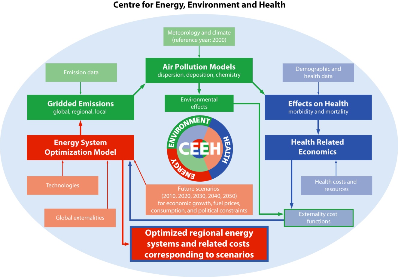
The purpose of this report is to describe the different components constituting the HIA-line in the CEEH integrated energy-environment-health-cost modelling. The CEEH framework consists of a number of independent models linked together to assess the impacts and associated costs of emissions from energy production on human health. The HIA-line carries out assessment of the health impact and associated costs of human exposure to air pollution from future scenarios for energy production in Denmark. The methodology employed is the impact pathway, where future emissions from all Danish air pollution sources are model ed in the Balmorel model; the emitted air pollution is then dispersed and chemically transformed in time and space by either the NERI or the DMI Atmospheric Chemical Transport models. The resulting concentration fields of air pollution are then averaged to give municipality based levels, and the resulting health impact and associated societal cost of the Danish population is modelled in the Health Impact Assessment model. The social costs associated with air pollution exposure are then converted from the modelled exposure costs to emission costs to be fed into the Balmorel model as additional energy production costs. The CEEH HIA-line presents a novel way of modelling health related consequences of air pollution, as it directly models, the demography, air pollution, morbidity and mortality, in a dynamic and integrated setup. When modelling the health impact of Danish emitted air pollution in the period from 2005 to 2030 we find 2,000 extra deaths of lung cancer, 3,950 deaths of heart disease, 7,375 deaths of stroke and 1,750 deaths of COPD, and 11.475 premature deaths, amounting to 163,075 lost life years in the modelled 25-year period. The health related social costs sums up to 60.8m € for lung cancer, 88.3m € for heart disease, 91.6m € for stroke, 18.7m € for COPD, 26.9m € for other cause mortality and in total 282.5m € throughout the period from 2005 to 2030. Page 4 of 63
Formålet med denne rapport er at beskrive "HIA-linjen" i den integrerede modelkæde af energi-miljø-helbred og omkostninger i CEEH. I CEEH er udviklet en række modeller, der i en samlet kæde kan estimere helbredskonsekvenser og heraf afledte samfundsmæssige omkostninger af udledning af luftforurening belyst ved scenarier for fremtidig energiproduktion i Danmark. Den anvendte metodologi kaldes "Impact Pathway", og består i en selvstændig modellering af alle fremtidige udledninger af luftforurening i Balmorel-modellen, en efterfølgende modellering af transport af og kemisk omdannelse af den udledte forurening i en af to forskellige Atmosfærisk Kemisk Transport modeller - enten NERI eller DMI-model en. De modellerede koncentrationsfelter, udglattes henover de 98 danske kommuner, og de resulterende helbredseffekter kan derefter beregnes i den udviklede sundhedskonsekvensmodel (Health Impact Assessment model). Dernæst kan de samfundsmæssige omkostninger beregnes og tilknyttes de i Balmorel-model en beregnede udledninger, således at der kan beregnes en samlet enhedsomkostning for luftforurening til brug for yderligere model eringer af fremtidig energiproduktion i Danmark. CEEH HIA-linjen præsenterer en ny måde at modellere og beregne samfundsmæssige helbredsomkostninger fra luftforurening på, i det der her direkte modelleres både demografisk udvikling, luftforurening og sygelighed og dødelighed i en integreret model. Modelleringen af de samlede helbreds konsekvenser ved dansk udledt luftforurening i perioden fra 2005 til 2030, giver 2.000 ekstra lungekræftdødsfald, 3.950 ekstra hjertesygdomsdødsfald, 7.375 dødsfald fra blodprop i hjernen, 1.750 KOL-dødsfald og 11,475 for tidlige dødsfald af andre årsager. Opgjort som tabte leveår finder vi et tab af 163.075 år i den modellerede 25 års periode. De samfundsmæssige omkostninger beløber sig i perioden til 456 mio. kr. for lungekræft, 662 mio. kr. for hjertesygdom, 687 mio. kr. for blodprop i hjernen, 140 mio. kr. for KOL, 202 mio. DKK for død af andre årsager, og i alt 2.149 mio. kr. i perioden fra 2005 to 2030. Page 5 of 63

Chapter 1. Overview of the CEEH modelling framework
1.1. CEEH framework
The CEEH framework (see methodological aspects in the CEEH-report number 1: Baklanov and Kaas, 2011) consists of a number of independent models linked together to assess the impacts and associated costs of emissions from energy production on human health. CEEH operates with two different model lines, the EVA-line and the HIA-line. This report presents the HIA-line; the EVA-line is presented in CEEH-report number 3: Brandt et al., 2011). Figure 1.1: Scheme of CEEH integrated model ing.
1.2. HIA-line in CEEH
The HIA-line carries out assessment of the health impact and associated costs of human exposure to air pollution from future scenarios for energy production in Denmark. The methodology employed is the impact pathway, where future emissions from all air pollution sources are modelled by the Balmorel model (Karlsson 2008); the emitted air pollution is then dispersed and transformed in time and space by Atmospheric Chemical Transport (ACT) models either DEHM or DMI-model (see chapter 4). The resulting concentration fields of air pollution, given in a detailed geographical grid, are then averaged to give municipality based levels, and the resulting health impact and associated societal cost on the Danish population is modelled in the Health Impact Assessment model. The air pollution exposure associated costs are then converted from exposure costs to emission costs and fed into the Balmorel model as additional energy production costs. Figure 1.1 depicts the major components and the data exchange in the CEEH modelling chain. Page 6 of 63
Chapter 2. Health Impact Assessment and modelling

2.1. Health impact assessment
Health impact assessment is a multidisciplinary setting, which aims to support policy and decision making by describing and evaluating the potential health impacts resulting from political decisions. In its broadest definition it covers a wide range of different methodologies from qualitative assessments made by expert opinion to more detailed and involved quantitative assessments typically based on various mathematical modelling strategies. 2.2. Health impact assessment modelling
Increasing computational ability makes it possible to develop dynamic quantitative HIA tools based on epidemiological evidence and with capacity to handle complex causality webs. Prevalence data on risk factor exposure is essential as well as disease incidence rates or mortality rates. Relative risks are the key parameters measuring the association between risk factors and diseases or death. HIA models that quantify the health benefit of intervention on lifestyle risk factors such as smoking, physical inactivity, unhealthy nutrition, obesity etc. have been developed during recent years. Most models have been developed to handle specific topics, but a few more generalised models exist and are being used in the field of health promotion and prevention of unhealthy lifestyles: Prevent, DYNAMO-HIA among others (Gunning-Schepers, 1989, Wolfson, 1994, Utley et al, 2003, Hoogenveen et al, 2010, Lhachimi et al, 2010, Lhachimi et al 2012). The main challenge of using HIA models that can handle exposure to structural factors such as environmental pollutants, climate changes, noise, and safe traffic, is that epidemiological quantification of the impact of these factors are generally not well established. Some HIA models are based on dynamic micro-simulation techniques and run individual life courses where shifts between states (e.g. unexposed, exposed, healthy, diseased and dead) operate by transition probabilities. The use of these models is limited because of scarce data. Other models operate on aggregated data and are often restricted as to their ability to handle different topics. In the CEEH framework, we have developed a new model with two aims: To be able to quantify the health impact on the Danish population of air pollution caused by Danish energy production, and to set up a framework for a general model with possibilities to assess health impacts on a wider range of policies or interventions affecting the Danish population. Page 7 of 63
Chapter 3. Description of the CEEH Health Impact Assessment model
The model developed within CEEH is a Multistate Markov Model combined with Monte Carlo methods and enables evaluating both the expected health impact and the uncertainties associated with a modelling methodology. The model is built around three parts, (1) a general demographic model including births and mortality, (2) an epidemiological modelling of exposure- and disease specific morbidity and mortality, and (3) a module to sum up resulting impacts and associated health costs. The model takes input from various sources, chemical species composition and geographical distribution of air pollution and the population, estimates of concentration-response associations between air pollution and morbidity and mortality, expected numbers of incident cases of morbidity and mortality from air pollution related diseases, and health and societal costs of incident cases of morbidity and mortality. A summary of input and output from the model is shown in figure 3.1. In order to model the Danish population over a period of more than 70 years, the model contains states corresponding to the demographic evolution and the included diseases, cause-specific deaths and mortality from other causes. The estimation of transition probabilities between states is made on the basis of linkage between nationwide registers (Thygesen and Ersbøll, 2011). When life course data from Danish registers and cohorts e.g. The Danish National Cohort Study (DANCOS) (Davidsen, 2011) are used, the actual estimation of transition probabilities can be made so that these fit in with conditions in Denmark and, thus, strengthen the model in two areas. Firstly, this strengthens the precision and validity of studies of treatments and interventions in Denmark and, secondly, it allows direct estimation of uncertainties in the transition probabilities, and afterwards inclusion of these uncertainties directly in the model as opposed to a traditional external sensitivity analysis. The impact of changed exposure is estimated through outcome measures obtained from the literature. The specific diseases associated with air pollution exposure included in the model simulations are cardiovascular and respiratory diseases as the evidence of associations with air pollution is most solid regarding these. Incidence rates are established from the Danish National Patient Register and the Cause of Death Register. The model does not take any potential effects of climate change, emissions of NH3 (dominated by the agricultural sector) or emissions from shipping into account. Page 8 of 63
Figure 3.1: Scheme of the CEEH Health Impact Assessment model (HIA-line)
3.1. Technical description
The Multi-state Markov Model is a framework, which models a dynamic population by partitioning it into a number of states and specifying a matrix of probabilities describing transitions between states as the time is moved forward in the model. The partitioning of individuals assumes that individuals in the same state have equal characteristics leading to equal transition probabilities for individuals in that state. In the model presented here different states corresponds to partitioning the population into age and sex specific categories of e.g. healthy people or people having a disease (figure 3.2). Thus, a Multi-state Markov Model is a very flexible framework, and the limit for detailing of the model is primarily determined by two factors: (1) which and especially how detailed data are available as to morbidity, co-morbidity, competing causes of death and parameters relating exposure and risk of disease, and (2) the amount of computer capacity available, as detailed models requires large amounts of computations. Page 9 of 63
Figure 3.2: Basic outline of the multi state Markov Model. Here shown with four states as circles, health, specific chronic
disease, cause specific death and death of other causes. The model starts with a 50 year old healthy individual, and
shows possible transitions as arrows.
In order to evaluate the impact of an intervention (i.e. changed exposure to air pollution), the model is run twice, once as a reference run without the effects of the intervention included, and secondly as an intervention run, where the effects of the changed exposure are factored in as changes in the risk of disease incidence. The impact of the intervention is then calculated as the output difference between the two model runs. The Monte Carlo method employed is a repeated run of the model over a number of years to get estimates of the uncertainties in the distribution of the population throughout the modelling period. By a number of model runs we can average outcomes to get a more precise estimate of the expected value of a particular outcome, and use the variability in outcomes to infer information on standard error of the expected value. The modelling is based on the described Multi-state Markov framework, built around the Danish population in the year 2010 disaggregated by gender, 1-year age groups and municipalities. For each of these combinations a number of states and transitions are available: Healthy (H), Incident Lung cancer (ILC), Lung cancer year 1 after incidence (LC1), Lung cancer year 2 after incidence (LC2), . , Lung cancer year 7 after incidence (LC7), Dead Lung cancer Incident year (DLCI), Dead Lung cancer other years (DLC), Incident Heart Disease (IHD), Heart Disease year 1 after incidence (HD1), . , Heart Disease year 9 (HD9), Dead Heart Disease Incident year (DHDI), Dead Heart Disease other years (DHD), Incident Stroke (IST), Stroke year 1 after incidence (ST1), . , Stroke year 9 after incidence (ST9), Dead Stroke Incident year (DSTI), Dead Stroke other years (DST), Incident COPD (ICOPD), COPD year 1 after incidence (HD1), . , COPD year 9 after incidence (HD9), Dead COPD Incident (DHDI), Dead COPD (DHD) and Dead Other Causes (DOC). This means that each person each year Page 10 of 63
will occupy one of the mentioned states, with transition probabilities (quite a few will typically be 0) characterising the possible states the person may occupy the following year. As the model has 8 states for Lung cancer (Incident case ILC, one year survivor LC1,., seven+ year survivor) and 10 states for Heart disease, Stroke and COPD (Incident case, one year survivor, ., nine+ year survivor) this means that persons surviving more than 7 or 10 years with Lung cancer or Heart disease, Stroke or COPD respectively will be kept in the final disease state until death. 3.2. Demography
Figure 3.3 shows the population prognosis for Denmark during the period for which CEEH makes projections. Marked changes in the population composition are seen, with more elderly and fewer young people. This is expected to affect the population's response to exposure to air pollution. The described Health Impact Assessment model takes these changes into consideration in the scenarios of the health consequences of air pollution. Figure 3.3: (a) the Danish population in 2007, by gender and 5-year age groups; (b) the projected Danish population in
2040, the broken line marking the population in 2007 by gender and 5-year age groups; Source: Statistics Denmark.
The demographic module handles the input from demographic forecasts of the Danish population during the years 1995 to 2050 to the model. The inclusion of a realistic demographic scenario for Denmark is based on already established projections (e.g. population prognoses from Statistics Denmark). On the basis of those, the model can then make deviations from established projections in two areas. Firstly, the model can operate on various breakdowns of the Danish population, for instance into the 99 municipalities, and be able to take into account gender and age specific population figures for single units in accordance with established projections. Secondly, the model can make changes in mortality and the resulting prerequisite conditions for population projections. In the CEEH model, the overall mortality in the Danish population has been projected for the period 2010 to 2040, by using the observed changes in overall mortality from 1995 to 2010 as a basis for a log-linear projection with each one-year-age-group having its own level, and projecting the development in five-year-age-groups. Furthermore we have made an assumption of a decrease of at Page 11 of 63
least 2 per cent pr. year in each age-group, as that is in line with the experienced increase in life expectancy of about 3 months per year for the last decades. Figure 3.4 compares the models population forecast with the Statistics Denmark population forecast for selected years. The projections are quite similar for the elder age groups. The differences in the younger age groups are because the model does not account adequately for migrations. Figure 3.4: Model ed populations at 2010 (red), 2020 (green), 2030 (blue) and 2040 (turquoise). Black lines are
corresponding forecasts from Statistics Denmark.
3.3. Epidemiology
On the basis of the demographic module the model calculates the impact of external health determinants and parameters of associations between risk factor exposures and morbidity and cause-specific death measured as either incidence of disease, number of hospital admissions, and number of deaths, life expectancy and quality-adjusted life-years (QALYs). In addition, the changes in mortality are reintegrated in the demographic model ing, and thus make the combined demographic and epidemiological model a dynamic tool for evaluation of health impact on a dynamic population under realistic assumptions. Disease Incidence Transition probabilities for transitions between the states Healthy and Lung cancer or Heart Disease, are based on calculations of disease incidence in Denmark in the years 1994 to 2006. The calculations have been made by merging information on the Danish population from Statistics Page 12 of 63

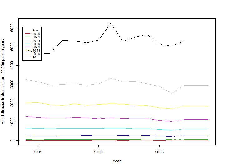
Denmark and the Civil Registration System, information on hospitalisations from the National Patient Register (Lynge, 2011) and information on deaths from the Causes of Death Register (Helweg-Larsen, 2011). By linking these registers it is possible to track hospitalisations on an individual level from 1977 to 2006, and for each person track their disease history in this period. This enables us to ensure that incidence calculations are only made on genuinely incident cases, and weed out possible inflation of incidence numbers by erroneously including re-hospitalisations. In addition we can distinguish between the main cause of hospitalisation and any other accompanying diagnoses. We are thus able for each disease to establish cohorts of all Danes who in year 1994 did not have had Lung Cancer, Heart Disease, Stroke or COPD, and follow these in the National Patient Register and the Causes of Death Register to determine the incidence rate of the diseases in the years following 2000. In addition the information in the Central Person Register ensures that immigration can be taken care of in the calculations. As we are following individuals in the cohorts the incidence rates can be calculated in sex and age specific strata to ensure a detailed model ing of the development of diseases in the Danish population throughout the modelling period. Figure 3.5 shows an example of disease incidence for male heart disease in 1994-2006, and the projection in 2007. Based on the observed incidence rates from 1994 to 2006, the average incidence rate discounted by 2% each year is used as the predicted rate in the modelling period, which ensures that the contribution to the overall mortality from the specifically modelled diseases is kept constant at a relative level, under the ongoing general increase in life expectancy as mentioned above. Figure 3.5: Observed (1994 to 2006) and predicted (2007-) incidence rates for male heart disease. Calculations are based
on 1994-2006 data from the National Patient Register and the Causes of death Register.
Page 13 of 63

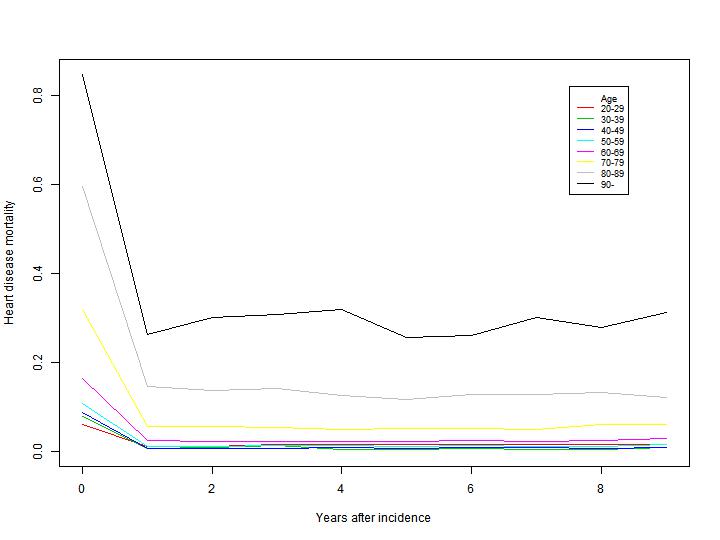
Cause specific mortality When following the cohorts described above, we can for all incident cases of disease determine date of disease (diagnosis) and if applicable date of death, and are thus able to calculate disease specific death rates, to use as transition probabilities for transitions between the various disease and death states included in the model. We can then calculate mortality rates for each year following incidence, to model the development of mortality as a function of both age and time since incidence of disease. Figure 3.6 shows an example of calculated death probabilities in the years following incident heart disease for males based on 1994-2006 data. The unique possibilities of register linkage in Denmark enable us to do these calculations in detailed sex and age strata. Figure 3.6: Observed probability of dying for men by years after heart disease incidence. Calculations are based on 1994-
2006 data from the National Patient Register and the Causes of death Register.
Other cause mortality When modelling specific diseases and cause specific mortality we need to adjust the total mortality to avoid double counting of deaths. The detailed level of information in the Danish Registers makes it possible to partition the total mortality into a directly modelled part from the included diseases, and an indirectly modelled part, which covers all other causes. Page 14 of 63

Exposure and changes in transition probabilities A change in exposure to air pollution gives rise to a change in risk of developing disease or dying, which in the Multi State Markov setup is modelled as a change in transition probabilities between the healthy state and one or more disease or death states. The actual change in probabilities depends both on the level of change in exposure, and on the level of association between exposure and disease or death. In CEEH the size of change in exposure is modelled by the ATC-models (see chapter 4), and the association between exposure and disease or death is measured by relative risks taken from the literature on air pollution and health impacts (see chapter 5). 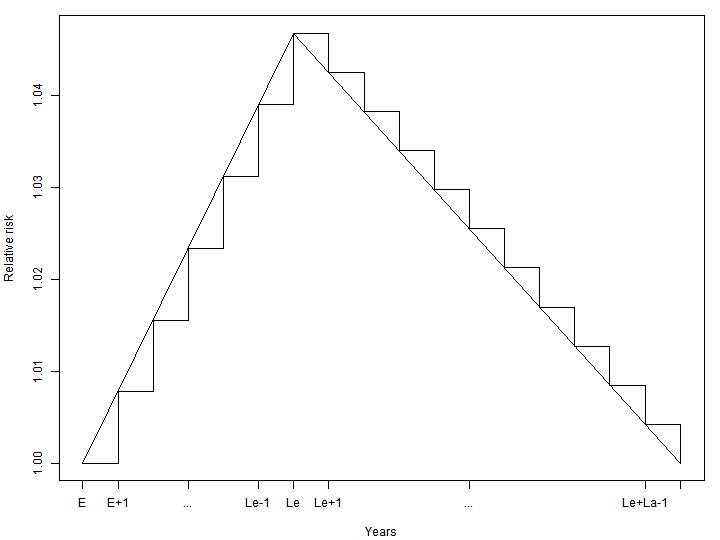In order to model the disease and mortality processes adequately in time, the model takes into account two disease specific parameters, lead time (time from exposure to maximum disease incidence risk increase) and lag time (time from maximum disease incidence risk increase to no risk increase again), and partitions the change in relative risk from an exposure at a given year into relative risk changes the following lead + lag years. Figure 3.7 shows an example of an increased relative risk partitioned into partial increases in the years following an exposure episode (e.g. air pollution emissions from a single year). The risk increases linearly from the exposure year to the lead time year, and then decreases linearly again until lag years have passed since lead time. Figure 3.7: Partitioning of increased relative risk in years following exposure. E denotes exposure year, Le lead time and
La lag time.
Page 15 of 63
3.4. Outcome measures
The combined demographic and epidemiological modules calculate a number of health impact outputs and associated uncertainties, e.g. number and year of excess incident cases, number and years of excess years with illness, number and year of excess deaths. Based on these, summary measures of health impact (lost life years, life expectancy) can be computed, with confidence intervals. Economic Module The aim is, on the basis of the health outcomes from the impact modelling, to quantify the resource use and cost of changes in morbidity and mortality. This wil be done in a framework of attributable cost, where the costs associated with pollution related diseases are calculated as the difference in average cost for persons with and without the specific disease. The cost will focus on resources used to treatment and care in the primary and secondary health care service, and consequences for social production. Potential costs and savings from avoided premature deaths will also be estimated, as will the health care cost during the last life-year (see chapter 6). To enable calculations of net present values three different discount rates (0%, 3% and 5%, 3% are used in the Energy system modeling) are used to convert future costs into present costs. In that way, the economic module can provide unit costs of emissions to use in the integrated CEEH model chain, and the HIA-line can be applied to make cost-effectiveness analyses of scenarios for future Danish energy production and the resulting air pollution. 3.5. Validation
Tobacco smoking is a risk factor that has been studied for many years and the health impact from smoking is well documented (Stewart et al. 2008, Peto et al. 1992). A validation of the HIA model has been done by estimating the health effects of cigarette smoking and comparing the estimates with results from accomplished research. The validation is based on data reflecting the evolution that has already taken place in Denmark. Thus, model simulations are based on historical data on sex and age specific death rates for total mortality and lung cancer and prevalence data on smoking. Furthermore, the demographic changes are included in the test. As the relative risks from smoking on health are well established, these parameters are already available. The validation showed that the model performs in agreement with other recent HIA model studies of smoking. When model ing smoking behaviour in the male Danish population, we found a comparable number of prevented lung cancer cases (around 1000) as Soerjomataram et al. 2010. Brønnum-Hansen and Juel 2000 found an increase of 3.0 years in male life expectancy in 1995, if all smoking was prevented when using the method by Peto et al. 1992, which is in agreement with our finding of 3.44 years. The validation is documented in detail in Flachs et al, 2012. Page 16 of 63
Chapter 4. Exposure data from Atmospheric Chemical Transport
(ACT) models
4.1. Air pollution data
To assess concentration levels, spatial and temporal distributions of pollutants in the air for estimation of their population exposure and effects on human health, different dispersion and atmospheric chemical transport (ACT) models are used. Two main ACT modelling lines are realised within the CEEH modelling framework: the Danish Eulerian Hemispheric Model (DEHM), developed by National Environment Research Institute, Aarhus University (NERI), and the ACT-NWP modelling system, developed by the Danish Meteorological Institute (DMI). DEHM Atmospheric chemistry transport model
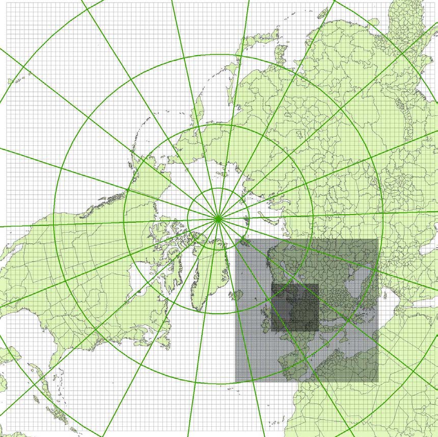
The Danish Eulerian Hemispheric Model (DEHM) (Christensen, 1997; Frohn et al., 2002; Brandt et
al., 2011) is a three-dimensional, offline, large-scale, Eulerian, atmospheric chemistry transport
model (ATC) developed to study long-range transport of air pollution in the Northern Hemisphere
(see figure 4.1). The model domain used in this work covers most of the Northern Hemisphere,
discretised on a polar stereographic projection, and includes a two-way nesting procedure with
several nests with higher resolution over Europe, and Northern Europe, the latter domain, which is
used in this report, is set up with a grid resolution of 16.67 km x 16.67 km.
The basic chemical scheme in DEHM includes 67 different species based on emissions of e.g. SOx, NOx, VOCs, NHx PM and CO. The current model describes concentration fields of 58 photo-chemical compounds (including NOx, SOx, VOC, NHx, CO, etc.) and 9 classes of particulate matter (PM2.5, PM10, TSP, sea-salt < 2.5 µm, sea-salt > 2.5 µm, smoke from wood stoves, fresh black carbon, aged black carbon, and organic carbon). One of the particle classes, the fraction of sea-salt < 2.5 µm, is not yet implemented in the model. A total of 122 chemical reactions are included. Furthermore, the model has options for an additional chemical scheme for mercury (Hg) and a module for emissions and transport of persistent organic pollutants (POPs), including an extensive description of air-surface exchange of POPs for soil, water, vegetation and snow. The description of POPs and mercury is not a part of the results applied in the HIA line. The DEHM model is driven with meteorological data from the numerical weather prediction model MM5v3.7 model (Grell et al., 1995), driven by global data from National Centres of environmental Protection. Emissions are based on several inventories, including global emission databases used in the Northern Hemispheric domain, namely EDGAR2000 Fast track (Emission Database for Global Atmospheric Research; Olivier and Berdowski, 2001), GEIA (Global Emission Inventory Activity; Graedel et al., 1993) both with a 1° x 1° resolution and RCP (Representative Concentration Pathways) with a 0.5° x 0.5° resolution for historical data (Lamarque et al., 2010) and future scenarios (Clarke et al., 2007; Smith and Wigley 2006; Wise et al., 2009). Emissions from the EMEP expert database (European Monitoring and Evaluation Programme) with 50 km x 50 km resolution (Mareckova et al., 2008) are used in the nested domain over Europe. Page 17 of 63

Emissions for Denmark are based on the national emission inventory for NH3, NO2 and SO2 (http://www.dmu.dk/luft/emissioner/air-pollutants). For NH3 the basic spatial resolution is 100 m x 100 m which is then aggregated to the 50 km x 50 km grid. The temporal distribution of the ammonia emissions is calculated using a dynamical ammonia emission model (Skjøth et al., 2004, Gyldenkærne et al., 2005). For NO2 and SO2 the spatial resolution is 50 km x 50 km and the data include about 70 larger point sources. Ship emissions both around Denmark with very high resolution (Olesen et al., 2009) and global (Corbett and Fischbeck, 1997) are included. Figure 4.1: The DEHM model domain (polar stereographic projection) with two nests. The mother domain covers the
Northern Hemisphere with a resolution of 150 km × 150 km. The two nested domains included have resolution of 50 km
× 50 km and 16.67 km × 16.67 km, respectively.
With respect to emissions from natural sources, emissions from retrospective wildfires are included based on Schultz et al. (2008). The current version of DEHM includes the temporal allocation of emissions from the IGAC-GEIA biogenic emission model for biogenic isoprene (International Global Atmospheric Chemistry – Global Emission Inventory Activity; Guenther et al., 1995) as an in-line module. This module is being replaced by the Model of Emissions of Gases and Aerosols from Nature (MEGAN) (Guenther et al., 2006), however, this implementation was not available for the present Page 18 of 63
study. Natural emissions of NOx from lightning and soil as well as emissions of NH3 from soil/vegetation based on GEIA are also implemented in the model. The emissions in all domains are distributed in time and with height above the surface following patterns depending on the source categories. DMI Atmospheric chemistry transport models
Enviro-HIRLAM is an on-line coupled NWP (HIRLAM) and ACT model for research and forecasting of
meteorological as well as chemical weather (Baklanov et al., 2008, Korsholm, 2009b). The integrated
modelling system is developed by DMI and included by the European HIRLAM consortium as the
baseline system in the HIRLAM Chemical Branch (https://hirlam.org/trac/wiki). The model
description was done in (Baklanov et al., 2008; Korsholm, 2009b; Korsholm et al., 2009a).
The Enviro-HIRLAM contains parameterisations of the direct, semi-direct, first and second indirect effects of aerosols. Direct and semi-direct effects are realised by modification of Savijarvi radiation scheme (Savijärvi, 1990) with implementation of a new fast analytical SW and LW (2-stream approximation) transmittances, reflectances and absorptances (Nielsen et al., 2011). Simplified analytical parameterization for inclusion of direct aerosol effect on short-wave radiation was developed based on Koepke et al. (1997) using the DISORT model and considering the full spectral radiance field. The species include BC (soot), minerals (nucleus, accumulation, coarse and transported modes), sulphuric acid, sea salt (accumulation and coarse modes), "water soluble", and "water insoluble". Condensation, evaporation and autoconversion in warm clouds are considered to be fast relative to the model time step and are not treated prognostically. The bulk convection and cloud microphysics scheme STRACO (Sass, 2002) and the autoconversion scheme by Rasch and Kristjansson (1998) form the basis of the parameterisation of the second aerosol indirect effect. As aerosols are convected they may activate and contribute to the cloud droplet number concentration, thereby, decreasing the cloud droplet effective radius affecting autoconversion of warm cloud droplets into raindrops. Cloud radiation interactions are based on the cloud droplet effective radius (Wyser et al., 1999). As it decreases warm cloud droplet size and reflects more incoming short wave radiation, thereby, we parameterise the first aerosol indirect effect. A clean background cloud droplet number concentration is assumed and the anthropogenic contribution is calculated via the aerosol scheme. For long-term multi-year runs a more economical modelling system HIRLAM-CAMx is used. It is
Eulerian atmospheric chemistry transport CAMx (Comprehensive Air quality Model with extensions)
model) off-line coupled with the NWP DMI-HIRLAM model. There are
several gas-phase chemistry (RADM by Chang et al., 1987; CB4 by Gery et al., 1989; CB5 by Yarwood
et al., 2005b) and aerosol physics (2-mode CF and CMU sectional schemes, see CAMx Users Guide -
http://www.camx.com/Files/CAMxUsersGuide_v5-40.aspx) mechanisms available in the model
version 5.2. For the CEEH runs the CB4 with CF scheme were applied. All gas-phase mechanisms are
used together with the Tropospheric Ultraviolet and Visible radiation model (TUV) (Emery et al.,
2010) to calculate photolysis rate coefficients. Both CF and CMU algorithms include the following
processes: aqueous sulphate and nitrate formation in resolved cloud water using the RADM aqueous
chemistry algorithm (Chang et al., 1987); partitioning of condensable organic gases to secondary
organic aerosols (Strader et al., 1999); partitioning of inorganic aerosol constituents (sulfate, nitrate,
Page 19 of 63

ammonium, sodium, and chloride) between the gas and aerosol phases using the ISORROPIA thermodynamic module (Nenes et al., 1998, 1999). CAMx has two dry deposition options for both gases and aerosols: the original approach based on the work of Wesely (1989) and Slinn and Slinn (1980); and an updated approach based on the work of Zhang et al. (2001; 2003). The horizontal and vertical resolutions of the model depend on resolutions of the meteorological and emission data. At present the model runs over a 0.2º×0.2º horizontal grid, and it has a vertical resolution of 25 levels covering the lowest 3 km of the troposphere. The amount of chemical compounds, which is transported from the free troposphere into the atmospheric boundary layer, is determined by the meteorological information and the concentration of the chemical compounds in the free troposphere. These concentrations depend on the longitude, latitude, land/sea and month. The advection equations are solved be the Piecewise Parabolic Method (PPM) of Colella and Woodward (1984) as implemented by Odman and Ingram (1993). All HIRLAM-CAMx computations for CEEH are forced by ECMWF meteorological data, chemical BCs/ICs from DEHM and TNO anthropogenic (Kuenen et al., 2010) as well as biogenic (calculated from DMI-HIRLAM output) emissions. The modeling domain covers Europe with horizontal grid resolution of 0.2 x 0.2 deg. and 25 vertical levels. 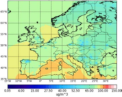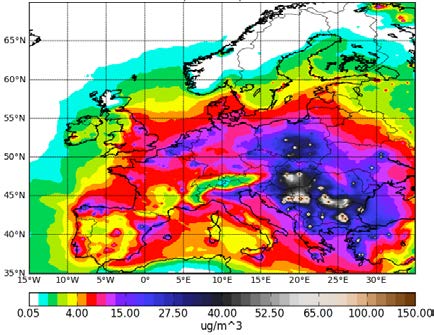Figure 4.2 shows HIRLAM-CAMx annual 2005 averaged contour plots of O3 and total PM2.5. High intensity emission sources in Paris, Rein Ruhr, Po Valley and other cities or industrial areas can be easily identified there. The O3 maximum values are 110 μg/m3 (Figure 4.2a), but regional background far from the Mediterranean area is twice less and equals to 50-60 μg/m3 with local minimum values of 10 μg/m3. The O3 sinks in major urban and industrial areas are attributed to high NO emissions (titration effects). The largest concentration of PM2.5 is 150 μg/m3 over Eastern Europe (Figure 4.2b), while the regional background concentration of anthropogenic aerosols is about 5-10 μg/m3. Figure 4.2: Annual mean concentrations of (a) O3 and (b) PM2.5 in μg /m3 for the year 2005 at the lowest HIRLAM-CAMx
model level.
Validation of the HIRLAM-CAMx model setup for CEEH versus the European air quality monitoring stations data for the year 2005 was done and published in the CEEH Report no. 8 (Kaas et al., 2012). Page 20 of 63
4.2. Transformation from geographical grid to municipalities
Since HIA is working in municipality units, the format of the air pollution data must be transformed from averages over grid areas into averages over the areas of the municipalities. The basic principle in this transformation is to determine the overlap areas between the grid areas and the individual municipalities. An average concentration over each municipality is then found by taking the average of the overlapping grid data weighted after overlapping area. In order to determine overlapping areas, the data are held in vector format, and the Matlab's mapping toolbox has been used. The ACT-model grid areas
The grid points takes (x,y) values corresponding to integer indices of a matrix of 96 x 96 points for DEHM and 251 x 176 points for HIRLAM-CAMx. Each grid data value is representing an average value over the area surrounding each grid point. A vector representation of each grid area was made up of a square bounded by x-0.5, x+0.5 and y-0.5, y+0.5. The longitude and latitude coordinates for the shifted grid were then evaluated. Figure 4.3 shows the distribution of PM2.5 (including primary and secondary particles - ammonium sulphates and ammonium nitrate) as modelled by the DEHM ACT-model. Figure 4.3: Increase in PM2.5 in year 2020 in the ACTM-grid in μg/m3.
The municipality data
Page 21 of 63
Geographical coordinates for the Danish administrative units, municipalities, can be found at the National Survey and Cadastre's (Kort og Matrikel Styrelsen) homepage: The data used here are vector data in shape format in 1:2 million's resolution. The data represent the administrative division of Denmark as of the "municipality reform 2007" with later changes and adjustments. The geographical coordinates are given in the UTM32 map projection with detailed information shown below given with the data. The data was read using the Matlap mapping toolbox. The UTM coordinates are transformed to longitude and latitude using a script "utm2deg" by Rafael Palacios, 2006. The script is based on WGS84 system, while the data coordinates are based on the EUREF89 system, which gives a negligible error of about 30cm on the coordinate transformation. Figure 4.4 is an example of transformed data, with pollutant PM2.5 distributed over the municipal grid. Combined figures 4.3 and 4.4 show how the transformation from ACT grid to municipal grid affects pollution levels only in a non-significant manner. Figure 4.4: Increase in PM2.5 in μg/m3 in year 2020 when transformed from ACT-model grid to averages at municipality
level. The scale (0-1) is relative, the absolute minimum (0.11) and maximum (0.63) is listed in the box.
Page 22 of 63
Chapter 5. Linking exposure and population health
The general approach to estimating the effects of pollutants on health uses the risk changes observed in epidemiological studies, expressed as % change in outcome per unit pollutant (concentration). If these concentration-response functions (CRF) are multiplied on the background rates of the health outcomes in the population at risk the CRF can be expressed as new cases (or events) per year (or day), per unit of this population, per relevant pollution increment. Results are then expressed as estimated additional cases, events or days per year attributed to the pollutant. The HIA-line operates with incidence rates for the diseases and calculates loss of life years from the incidence and typical course of the disease (assuming no difference in course between disease associated with air pollution and disease not associated with air pollution). Incidence is calculated as the percentage of the population for which a new episode of the effect occurs during a specific period and it typically refers to new episodes a disease but could also refer to cases of hospitalisation or death. The use of incidence of disease rather than total mortality is different from almost all other published approaches to calculate externalities of different emission scenarios as these have been based on large cohort studies of changes in prevalence of disease. The literature on changes in incidence rates associated with air pollution does not cover the entire spectrum of disease documented in prevalence studies and often use hospitalisation rates as a proxy for disease incidence. The question arises whether these can be used for calculation of incidence of the same diseases. In order to do this one has to assume that mild disease leading to contact with primary care only and severe disease leading to hospitalization is affected to the same extent by air pollution and that the risk for readmission is equal to the risk for first admission under the same diagnosis. It's unlikely that these assumptions hold true and that for some diseases the majority of incident cases are detected with delay when calculations are based on hospitalizations. It is known that the total of disease-specific causes of mortality does not sum up to the total overall mortality in cohort studies - an observation that is explained in part by the fact that diagnosis of diseases is less accurate than that of death and in part by the fact that many diseases may occur so rarely that statistical significance cannot realistically be reached in population studies. Thus the use of incidence-based concentration-response functions probably results in a significant but unknown underestimation of the impact of air pollution on health. In contrast to prevalence-based methods or inclusion of just premature deaths, the incidence based HIA method allows for accurate calculation of societal costs during the duration of disease including years of life lost. Based on a literature review, diseases were included in the HIA model if associated with air pollution and if they carry high societal costs either because they affect high proportions of the population or have very prolonged courses – thus generating high costs. Typically these are cardiopulmonary diseases. Rare diseases, diseases with weak associations with air pollutions, or a short duration among subjects within a short life-span (e.g. infants or elderly only) can only to a limited extent influence the societal costs of air pollution but were suggested for use in the model if associations were well documented and the risk of double counting (by inclusion in other broader categories of disease already covered) was considered negligible. Additionally, a 0.9% increase in cardiopulmonary Page 23 of 63
mortality per µg/m3 increase in PM2.5 was used for control of potential underestimation by use of the incidence-based CRF. See table Table 5.1 Recommended concentration-response functions for the HIA-line
Age & sex ICD-10 CRF (RR) Ozone Appendicitis K35.0 + 0.543% per 1 ppb Only during June-August K35.1 + increase in the K35.9 moving 5-day mean Ozone Asthma incidence PM2.5 Incidence of non-fatal I21-I25 + 2.4% per 1 μg/m3 cardiovascular events 50-79 yrs I61-I69 annual mean PM2.5 Respiratory hospital J00-J99 0.114 % per 1 μg/m3 Other than asthma among 2- admissions used as incidence 8 yrs and males 25+ yrs and COPD and lung cancer PM10 Ischemic heart disease I20-I25 0.08 % per 1 μg/m3 Only other than females 50- hospitalisation as incidence PM10 Dysrhythmia hospitalisation all ages I47-I49 0.08 % per 1 μg/m3 PM10 Heart Failure hospitalisation all ages 0.14 % per 1 μg/m3 used as incidence 36-64 yrs X60-84 0.326% per 1 μg/m3 moving 2-day mean Asthma incidence 8.75% per 1 μg/m3 Lung cancer incidence C33-C34 0.8 % per 1 μg/m3 0.467% per 1 μg/m3 J41-J44 0.0483% per 1 μg/m3 annual mean Otitis media incidence Children H65-H67 0.61% per 1 μg/m3 0-2 yrs PM2.5 Cardiopulmonary mortality 30+ yrs I10-70 + 0.9 % per 1 μg/m3 of Use to sum up total mortality J00-99 annual mean from disease specific CRF Page 24 of 63
The listed CRF includes some for specific diseases, age groups and gender and some that cover broad categories of diseases including the specific ones. When using the CRF for broad categories, the diseases and age groups already covered by use of specific diseases CRF should be subtracted as indicated in the notes. The HIA-line will include four different effects of air pollution: Cardiovascular diseases, Lung cancer, Stroke, Chronic Obstructive Lung Disease (COPD), and in addition an increase in overall mortality, which cannot be ascribed to the four specifically modelled diseases. Table 5.2 shows the identification in ICD-10 codes, the relative risks used as dose-effect functions between air pollution and disease incidence, and the lead and lag times used model the impact of air pollution in the HIA-modelling. Asthma among children is left out, as we cannot get valid estimates on incidence and duration, due to a lot of cases not being hospitalised, and thus not identifiable in the Danish registers. We note, that this is has potential to influence the effect of air pollution, as disease among children is likely to affect their parents labour market attachment or productive efficiency, and thus incur social costs at a non-discernible level. The chosen methodology however does not allow us to estimate these. Table 5.2: Included diseases, ICD-10 codes for identification and relatives risks and lead and lag times as used in the HIA-
modeling of air pol ution.
ICD-10 coding Relative risk for Relative risk for Lung cancer C33 - C34 I20 – I25 (410- I60 – I69 (430- J41 – J44 (491- Page 25 of 63
Chapter 6. Cost of morbidity and mortality
In this chapter we describe, the nature of the different assumptions relating to the resource use and costs applied in the HIA-model, and how we have derived these assumptions for costs of different patient groups. Some of the analyses have already been reported in journal articles where a thorough and more detailed description of the analytical process has been documented (Sætterstrøm et al., 2012, Kruse et al. 2012). Below is a brief description of the theoretical framework for describing the social cost of health consequences associated with air pollution. The scientific literature provides good evidence that a higher level of air pollution is associated with increased risk of mortality and morbidity from a variety of diseases. To the extent that a reduction in air pollution is related to a reduced risk of disease and severity of disease and thus potentially improves population health, it is likely that some health economic benefits arise in terms of better and/or longer life, a lower use of health care resources and an increase in social production. However, individuals who live longer and healthier lives also have increased general consumption of food, housing transport and other modern life conveniences. Economic analyses and especially evaluations of interventions aimed at reducing the level of air pollution, should ideally consider all changes in resource consumption no matter where and when they arise. Such perspectives are used in the traditional cost-benefit framework conducted from a social view point. A change in the level or distribution of air pollution may be introduced from political decisions (e.g. a decision to invest more power production from windmills/solar power rather than from coal or other polluting technologies) or from the a general developments over time (e.g. changes in power demands, traffic patterns, population composition and position), or from changes in the production industry and population's general behaviour and behaviour in relation to energy consumption in particular). One aim of the HIA model is to develop a tool that enables the analysis of the economic consequences of such interventions. The economic consequences of implementing intervention/policy change include the resource use and cost associated with such implementations. For example, these costs may include the cost associated with developing new power plants and replacing the old ones. All additional use of resources related to such developments may be termed as the intervention costs. The intervention costs are associated with each scenario of air pollution and will not be modelled by the HIA, although the cost should be included in the overall assessment of the cost-benefit of the particular scenario. For the full CEEH chain optimizations, however, such costs are included in the Balmorel model as mentioned in section 1.2. The intervention may result in reduced levels of air pollution (direct effect), which may affect the population health and occurrence of different diseases (fewer individuals with the disease, more individuals with less severe diseases). Reductions in the morbidity and mortality will have consequences for the demand for health care services and for the cost of the health care sector. Health care may be defined broader than just hospital care, but should also include less consumption of services in the primary sector (doctors, drugs), and often the primary municipal nursing and privately provided health care and support. Page 26 of 63
The HIA model is developed to model such relations and to provide estimates of the number of individuals with different disease and their survival. The cost part of the model applies assumed cost data to the changed number of people and life-years with different diseases, and aggregates the total health care cost associated with the changed morbidity pattern. A special consideration is the health care resource use and costs during the last period of life. This is a period where many individuals have great use of health care. If an intervention is successful in extending the life time of some individuals it means that they may have a longer period without serious illness and that the health care cost associated with conditions and illnesses near death are postponed. This will influence the timing of the resource use and perhaps also the amount of resource use. In a cost benefit framework a reduction in disease prevalence and severity and improvement in longevity is associated with a social value and considered as a benefit. One approach of such social valuation would be to describe the changes in health in terms of Quality Adjusted Life-Years (QALYs). In this approach, social values are assigned to the health state of the population and its survival. Such valuations are controversial and there exist different principles and different methodological strategies to obtain such valuations. Another approach would be that of the human capital method, where the consequences of changed population health is described in terms of contributions to social production. In this approach it is assumed that the value of avoided illness and longer survival should be valued according to a measure of production. If an intervention, for example is able to reduce the mortality of 40 year old men, then the human capital principle would determine the social valuation of such a health improvement as the additional social production these men would be able to contribute in their remaining life time. The production gain could then be measured as well as the gain in gross salary (as an approximation of the value of their production) these men would have until they retire from the labour market at their age of pension. Gains in production value may arise from both more time in the labour market and from higher production (salaries) at the labour market. The friction cost method is a special application in situations where the human resources are not used to social production (unemployment). Friction cost applications only consider the lost production during the transition period, i.e. the period where one person has left a work place until that person has been replaced by another person. A third approach would be to aggregate the intrinsic value of gained life or life-years which is applied in the EVA-line of the CEEH (Brandt et al., 2011). Such approaches apply valuations of life or life-years obtained from so called "willingness to pay" studies. This approach assumes, that it is possible to obtain assessments of valuation of life through survey studies, where respondents are asked to place monetary values on small changes in risk of deaths (e.g. from improved traffic control/seat belts) and from such replies model the valuation of life. Valuations of life-years would be based on assumed valuations of life, assumptions of the remaining life time of such life and assumption of time preferences (discount rate). Analyses of intrinsic valuations are highly controversial due to the many assumptions required and several review studies have indicated that the variation in the value of life (and life-years) have huge variations (Doucouliagos et al. 2012, Lindhjem et al., 2011, Rausser et al. 2011). Page 27 of 63
The structure of the chapter is as follows. In the subsequent sections these different aspects of the applied costing methods are described. The first section focuses on the identification of relevant individuals on whom we base our cost estimation. The second section reports on the unit cost for the health care resource consumptions for the two main diseases that are affected by air pollution (lung cancer and cardiopulmonary disease). The third section reports on health care cost during the last year before death, which is a period with high use of health care resources. The fourth section reports on cost related to labour market consequences associated with cardiopulmonary disease. The fifth section describes how the effects of disease might influence the affected individuals' health related quality of life. The sixth section describes assumptions in relation to consumption of other resources than health care. The last section describes assumptions relating to valuation of avoided deaths and life-years lost. 6.1. Identification of individuals with disease
In the HIA-cost analysis we have focused on two major groups of diseases where reliable evidence appears to indicate a clear association with air pollution, namely lung cancer and cardiopulmonary disease. For the costing studies we have identified individuals with these two diseases based on data from the National Patient Register from 1977-2006 and the Causes of Death Register. The National Patient Register holds information about all resident Danes' use of hospital services (Lynge, 2011) and the Causes of Death Register holds information about all resident and deceased Danes' cause of death. The relevant diseases were defined according to the International Classification of Diseases version 10 (ICD-10). In the database available for this project, the hospital data were arranged in yearly data files. Each file included encrypted personal identification number (The unique Danish Civil Registration system identification), diagnostic codes, hospital admission record id, ICD-10 code and type of diagnostic code. The Causes of Death Register was arranged as one file for the entire period. It included encrypted personal identification number (The unique Danish Civil Registration system identification), ICD-10 code for cause of death and date of death. Each hospital record might include several diagnostic codes and for this analysis we had access to both the primary discharge diagnosis as well as supplementary diagnoses. An individual with one of the relevant diseases was defined as a person who in the observation period had at least one hospital contact (inpatient or outpatient), which was coded with the disease as the primary diagnosis or who died with the disease coded as cause of death. We assumed that the first recorded diagnosis defined the onset time of the disease. Thus, the identification of diseased individuals was based on the assumption that a patient is an individual with the disease, if a hospital doctor once during the observation period has diagnosed the patient with the disease or if the patient has been recorded to die from the disease. This will lead to a lag in disease incidences, particularly for diseases with a long pre-hospital phase, such as COPD, we do not however have other possibilities for getting population wide information on disease incidences. Page 28 of 63
From the sample of individuals with the relevant diseases, only those who were alive at January 1st 1997 and who had had no previous diagnosis with that disease were included in the cost analysis. The sample of patients included individuals who died during the observation period. This group was handled in separate analyses in the healthcare cost analysis and the productivity analysis. 6.2. Health care costs for diseases related to air pollution
Consistent cost data were available for the years 1997-2006. 1997 was the first year where data from the primary sector were available. The cost of health care services were assigned according to the national DRG-system for hospital contacts (inpatients and outpatient) and by the fees paid by the social health insurance for services rendered by the primary health care providers. The use of hospital resources was defined in terms of numbers of hospital contacts. A contact can take place as a visit at the emergency room, an outpatient contact or as an inpatient admission. For each contact there is a description of the resource use associated with the contact based on the Danish national diagnostic related group-system (DRG). Resource use in the primary care sector was defined in terms of services provided by primary care providers who received a fee from the public health insurance system. The primary health care sector includes general practitioners, practicing specialists, dentists, physiotherapists, chiropractors and others. Each service provided was associated with a fee paid to the provider. This fee can be interpreted as a proxy for the value of the use of resources for the service. However, the fee structure was negotiated between the provider and purchaser organisations and does not necessarily reflect the true cost of the service. Use of medication was valued as the full prise charged by the pharmacy including prescription charge but excluding value added tax. To analyse the health care cost of a long-term disease the cost data were assigned to yearly time intervals defined from the calendar year of the first diagnosis. When the cohorts were identified in 1997 (for cardiopulmonary disease) and 1997-2003 (for lung cancer) there were thus up to 10 years of follow-up cost data for cardiopulmonary disease and 4 years follow-up for lung cancer. The analytical data consisted of cost data for the cohort of individuals with disease in the given year (cases) and a group of individuals without the disease matched in a 1 to 5 relation (five controls for each case). The average health care costs for these two cohorts were estimated: one average yearly cost for cases and one for controls. These estimates were computed on the basis of individuals who were alive at the beginning of the year. The difference in average yearly costs for the two cohorts was defined as the attributable cost of the disease, i.e. the additional cost associated with the disease. The aggregated average cost for each considered year discounted can be interpreted as the net present value of cost for hospital care and primary care combined. Page 29 of 63
In the analysis we stratified the cost data according to gender and age (in five year intervals) as shown in Tables 6.1-6.4. Table 6.1: Discounted attributable healthcare costs, lung cancer, men (DKK), 1997-prices
0 235.209 209.149 177.647 164.746 119.747 109.290 76.475 1 42.675 30.294 23.605 14.612 -7.611 -10.383 -11.817 -7.986 -10.828 -11.818 -12.097 Net 279.924 236.793 195.490 167.368 109.997 91.769 44.176 Discounting was made at an annual discount rate of 3 per cent.
Table 6.2: Discounted attributable healthcare costs, lung cancer, women (DKK), 1997-prices
0 213.593 190.563 185.075 179.884 136.710 100.269 77.626 1 26.769 24.026 32.093 14.602 -3.709 -10.320 -10.480 -6.572 -12.136 -11.784 Net 240.219 216.924 210.862 187.407 136.053 78.216 48.809 Discounting was made at an annual discount rate of 3 per cent.
Table 6.3: Discounted attributable healthcare costs, cardiopulmonary disease, men (DKK), 1997-prices
Page 30 of 63
26.430 58.378 77.196 86.036 107.693 103.024 100.878 111.170 9.174 11.759 12.288 17.973 18.762 13.210 11.150 47.181 111.123 138.317 161.362 189.789 181.797 161.969 134.338 Discounting was made at an annual discount rate of 3 per cent. Page 31 of 63
Table 6.4: Discounted attributable healthcare costs, cardiopulmonary disease, women (DKK), 1997-prices
0 22.008 38.137 44.203 59.277 72.320 86.121 104.681 119.745 1 3.479 6.363 8.070 12.565 11.279 13.415 15.813 11.676 2.402 4.054 4.301 2.438 3.726 5.023 2.152 3.735 4.868 2.197 4.189 4.710 2.375 4.257 5.657 2.445 4.503 5.578 2.594 5.236 5.863 2.459 4.989 6.142 Net 44.549 79.189 94.414 129.880 146.360 155.639 168.514 139.005 Discounting was made at an annual discount rate of 3 per cent. The applied methods, calculations and results are further documented in Sætterstrøm et al, 2012. 6.3. Healthcare costs in the last period of life
As mentioned previously most of the mortality related to air pollution relates to either lung cancer or cardiopulmonary disease. A share of pollution-related mortality, equal to the difference between pollution-related all cause mortality and pollution-related mortality caused by lung cancer and cardiopulmonary disease has not been accounted for in the approach describe above. We regarded a change in mortality to longer survival as a shift of healthcare costs into the future. To value the health care cost associated with postponed mortality, we calculated the average healthcare cost in the last half year of life stratified by gender and age in five-year intervals. These healthcare costs are then used as input to the HIA model and attributed to a deaths not related to lung cancer or cardiopulmonary disease. The study population was defined as Danes who died anytime during 2006, where death was not caused by lung cancer or cardiopulmonary disease (inspection of register for cause of mortality) and where the deceased has never been diagnosed with either of the two diseases (inspection of national patient register). The cost data used for this analysis included hospital care and primary care as well as pharmaceuticals prescribed. The costs of pharmaceuticals were restricted to the registrations of pharmacological treatments provided by the primary care pharmacists. Medications provided by the hospitals are included in the hospital care cost, and were not included in the primary care pharmaceuticals. The pharmaceutical cost entails the full cost of the purchase including own payment, reimbursements and shares paid by health insurance. Page 32 of 63
Table 6.5: Healthcare costs in the last half year alive, 2006-prices (DKK)
Men 109.998 119.737 139.949 122.034 137.071 118.811 Women 135.250 154.590 158.786 157.746 133.264 106.992 81.812 45.789 Methods, calculations and results are further documented in Sætterstrøm et al, 2012. 6.4. Labour market consequences
The labour market consequences of diseases related to air pollution were analysed using the human capital approach. If an individual deceases or leaves the labour market prematurely due to disease, then it is assumed that a productivity loss occurred in the year of this event and all subsequent years until s/he would otherwise have left the labour market (pension age). The productivity losses during the subsequent years were discounted to the net present value at the year of leaving the labour market. This approach does not distinguish between death and labour market withdrawal alive. Another labour market consequence of disease is the relative wage loss arising from a diseased person being absent from work for longer periods or choosing to work part-time. The wage loss is computed as the difference in wage development of patients with the wage development of a comparable reference group. This analysis did however render insignificant results of small magnitude and are not reported here. In addition disease in children will incur labour market absence for parents, and this might make a significant contribution. It is not possible however to infer valid estimates of incidences of e.g. asthma among children from the population wide registers, as many children with asthma are not hospitalised, and thus not registered. For computation of the productivity loss of patients leaving the labour market prematurely, a similar approach was applied as was used in the calculation of health care costs (cf. above). All individuals in the labour market leave the labour market at some point in time. The focus of the analysis was therefore to ascertain whether patients with the relevant diseases leave the labour market earlier than they would have done otherwise. To describe what the patient group would have done if they had not had the disease, we compared the patient group's labour market behaviour with that of a reference group. The reference group was composed to be comparable to the patient group with consideration of all features that possibly could influence mortality and labour market behaviour. The reference group was identified by matching on the following variables: gender, age, age squared, educational level, marital status, national origin, job function, residential area (urban/rural), co-morbidities and predicted smoking status. We applied the propensity score framework, cf. above, and matched five controls per case by ‘nearest neighbour'. The cohorts of patients and matched controls were restricted to include those who were at baseline were attached to the labour market (the year before incidence of disease). We used Cox proportional hazards model to analyse whether individuals with the two considered diseases leave the labour market earlier than individuals in the control group. The analyses showed, that patients Page 33 of 63
with cardiopulmonary disease leave the labour market earlier (due to death or early retirement) than their controls. The increased risk of leaving the labour market was multiplied with the average wage for cardiopulmonary diseases and discounted to the incidence year (1999). These computations were done until pension ages 65 (i.e. the current age of retirement) and 60 (the current age of early retirement) and a variable pension age (reflecting a recent government ruling). The data in Table 6.6 includes net value productivity cost for individuals with cardiopulmonary disease only. Most lung cancer patients were older than 65, and we did not find any statistically significant productivity loss for these patients. Table 6.6: Productivity costs, cardiopulmonary disease, NPV, fixed 2000 DKK prices
113,208 101,227 118,931 282,183 239,112 291,424 235,902 200,346 239,869 164,764 144,826 168,410 348,392 161,852 348,392 167,568 107,599 167,568 In addition to the disease related productivity cost, there appears to be an additional productivity effect relating to death from other causes. An analysis of the productivity cost related to "additional mortality" will have a number of methodological weaknesses. The analyses of health care costs and productivity costs all are based on identification of individuals with a given pollution-related disease, and a relevant control group. It was not possible to identify individuals dying from these unknown causes. Neither was it possible to identify the group of "unknown causes". Therefore, it was not possible to compute attributable health care costs or increased risk of leaving the labour market for this unspecified group. For similar reasons, it was not possible to compute the remaining time in the labour market due to lacking information of the age of these individuals. Thus, the labour market consequence for this residual group of individuals, we can only identify an average productivity cost in the year of diagnosis. This was estimated at 305,868 DKK for men and 244,252 DKK for women (2009 prices). Methods, calculations and results are documented in Kruse et al, 2012. 6.5. Health Related Quality of Life associated with disease
Different diseases have different impact on peoples' life. Health related quality of life (HRQOL) is a concept that is often used in health economics analyses to indicate the functional and social Page 34 of 63
consequence of diseases. A wide range of survey instruments have been developed to describe HRQOL and changes in HRQOL. In economic evaluations it is often desirable to compare the consequences of interventions across different diseases. Such comparisons require instruments that are able to capture relevant aspects of peoples' functional and social status independent of the disease they encounter. Generic HRQOL instruments have been developed to comply with such requirements and are in this respect different from disease specific HRQOL instruments. Most HRQOL instruments describe health status as a profile of scores in different dimensions (e.g. status of physical function, ability to maintain own care, ability to undertake usual activities, pain and discomfort, and mental health). Some generic instruments can be converted to a preference index measure of health status. Ideally, such an index should describe the value (utility) of a particular health status for example on a scale ranging 0-1 where 0 indicates death and 1 full health. In economic analysis it is customary to describe the effect of an intervention in terms of changes in life expectancies (gain in life years) and changes in HRQOL (gain in quality of life) in a combined measure of quality-adjusted life years (QALYs). 1 QALY indicate a full life year with perfect health status. The QALY indicator enables comparisons and trade-offs between gains in life time and gains in health status. There exist several such generic HRQOL instruments that can derive index scores. A relatively simple and commonly used instrument is the EQ-5D that describes health status in five dimensions (mobility, self-care, usual activities, pain and discomfort, anxiety and depression). Each dimension is described in three levels (no problems, some problems, extreme problems). There exists a validated Danish version of the instrument, a recommended Danish scoring algorithm and Danish population norm data. Another instrument is the 15D. This is also a generic instrument with a validated Danish translation and a scoring algorithm. This instrument includes 15 health dimensions where each dimension is described in five levels. A third example is the SF-6D instrument that can be derived from the more commonly used SF-36 and SF-12 questionnaires. Two strategies have been employed to describe the consequences on HRQOL of diseases related to air pollution. One is based on a review of the literature and inspection of publicly available sources. The second is based on analysis of the Danish health and sickness survey from the National Institute of Public Health. The Tufs Centre for the Evaluation of Value and Risk in Health, at the Institute for Clinical Research and Health Policy Studies, Boston maintains a registry of utility indices for different diseases. A search in this registry identified the following scores: Cardiopulmonary disease The utility of survivor's cardio pulmonary resuscitation scored 0.75 (Nichol et al., 2009), while in other study individuals with Pre-CABG scored 0.574 and 6 months post CABG (cardiopulmonary bypass pump) scored 0.658 (Al-Ruzzeh et al., 2008) Page 35 of 63
A recent study analysed the HRQOL index of lung cancer (Gordon et al., 2010). Individuals with no lung cancer scored 1, while individuals with early stage lung cancer (I and II) scored 0.73 and individuals with advanced stage lung cancer (III & IV) scored 0.66. Thus the impact of lung cancer was thus estimated at a HRQOL loss of 0.27 for early stage and 0.34 for advanced stage. Other studies have found HRQOL indexes of 0.75 (Liinden, 2010) and 0.47 (Asukai, 2010). Based on a large Finish population health survey the marginal effects of pulmonary disorders and cardiovascular disorders were estimated as outlined in the table. Table 6.7. Marginal effects of conditions on health utility measured with 15D and EQ-5D, adjusted for socioeconomic
factors and other conditions.
Pulmonary disorder Cardiovascular disord. -0,006 Pulmonary disorder Cardiovascular disord. -0,021 Source: Saarni et al, 2007. 6.6. Consumption of other resources
It is difficult to ascertain the consumption of the population and variations for different groups of the population. For this analyse we have applied an estimate for average yearly consumption per inhabitant without any variation according to gender, age or social groups. It was desirable to have an estimate that was relevant for Denmark. According to Statistics Denmark the private consumption excluding auto vehicles were 349 billion DKK in 2010 (Statistikbanken, NATK03). The population size was 5.6 million thus the average annual private consumption per inhabitant was about 62.400 DKK. 6.7. Value of lost life and life-years
The value of life is a topic of considerably scientific interest. A large meta-analysis has been conducted by the OECD reviewing stated preference studies with focus on the environment, transport and health sectors (Lindhjem et al, 2009). Based on nearly 900 observations, they estimated mean values of statistical life in 2005 purchasing adjusted US-$ of 6.3 mio. 400 observations were within the range of 0-2.5 mio US-$ while more than 150 observations fell within 2.5-5.0 mio US-$. Page 36 of 63
There exists only few reliable Danish assessment of the value of life. A Danish ph.d.-study focusing on value of life within the traffic sector derived at an valuation of 12-18m DKK per life dependent of different estimation methods (price level 1993) (Kidholm, 1996). In cost-benefit analysis the value of a life-year gained is often described as the average gross domestic production per person. The Danish GDP per capita in 2010 is shown in the table below. The average GPD per person was about 300,000 DDK in 2009 which is the latest year with available data. Table 6.8 GDP per capital (current prices, DKK)
Source: Statistikbanken, NAT15 The HIA-line only models social economic costs consisting of health care costs and production losses as described in chapter 6, and do not include valuations of lost life or lost life years. 6.8 Discussion of the unit costs
In this part of the report we have described how we have obtained different unit costs for the elements included in the HIA model. No matter how comprehensive and valid data such calculations are based upon, a number of implicit and explicit assumptions will influence the estimation of unit cost and their validity. For the purpose of the HIA model we have aimed at obtaining cost data that reflect long-term average cost, and apply such unit costs to model the health care resource consequence of different energy scenarios. In our cost estimates we have included large groups of resource uses but due to lack of reliable data some resource use have not been included. This applies for example to resource provided by the municipal health care services (home help and support) and support provided by voluntary organisations and the patients' families. Further, we have not included the time cost of patients related to treatment or wider implication on children and families of diseased adults. From a theoretical viewpoint the costs should ideally reflect society's opportunity cost, i.e. the utility that is forgone from the second best application of resources. There may be many reasons why the long-term average cost is not a good approximation of the opportunity cost. In our analysis we have assumed a fixed level of capacity (hospital and other infrastructure) which means the fixed cost element may not be fully included in our estimates. The cost data provided here assume that no expansion or extraction of such capacity will be required and that the changes in demand can be accomplished within the given capacity of the health care sector. It is assumed that the marginal cost of an expansion is identical from the marginal saving of a reduction. This is not necessarily true. If more services are required (and the production is close full Page 37 of 63
capacity) then an expansion would be associated with higher costs than the long-term average cost, and the cost might therefore be underestimated. However, if less services are required it might be difficult to realise the full savings as indicated by the long-term average cost since that may require discretionary capacity reduction (closure of whole hospital units) to realise the full saving. The cost estimates assumes a certain level of economics to scale. This may not be achievable with (large) reductions in service demanded (assuming lower use of the fixed capacity). This would lead to an overestimation of the potential saving. Applying the cost estimates in a long-term time perspective meets a further set of challenges, namely that medical technology develops over time. Such developments may make the treatment technology more expensive (new technology), more efficient (good use of capacity and routine skills) and cheaper (new cheaper technologies may replace and old expensive). It is difficult to assess the likely consequences of future technology development. Also the future demand for health service is difficult to predict. Now diseases may arise (e.g. AIDS), old ones vanish (e.g. Tuberculosis), new life styles may put greater emphasis on treatment of certain diseases (.e.g. a more obese population may have higher prevalence of diabetes) and therefore have influence on the use of health care resources. The political prioritisation of public resources to the health care sector may change and result in more (or less) resources being allocated to health care. Consequently, there are many uncertainties related to the cost elements of the HIA model. Page 38 of 63
Chapter 7. Results
7.1. Air pollution modelling for 2005 to 2030.
We have modelled the health effects of all Danish emission in the years 2005 to 2030 including all sectors (snap codes 1 – 10: Central power and heating plants, Domestic decentralised heating, Combustion in manufacturing industry, Production processes, Extraction and distribution of fossil fuels and geothermal energy, Solvents and other product use, Road transport, Other mobile sources and machinery, Waste handling and incineration, Agriculture). The ambient pollutants modelled are PM2.5 (primary), NO3, SO4 and NO2. Figure 7.1 and 7.2 shows as an example the distribution of air pollution (PM2.5 in year 2005, from local heating, wood stoves etc.) across Denmark as modelled by the DEHM ACT-model (figure 7.1) and when calculated according to municipalities for input to the HIA-model (figure 7.2). Figure 7.1: PM2.5, concentrations as modeled by the DEHM model, for al Danish sources in year 2005.
As the DEMH ACT-model simulated only a discrete series of individual years (2005, 2020, 2030, 2040 and 2050) with different emissions for each year, we have interpolated air pollution in years lying between 2005, 2020 and 2030 linearly. It is noted that for the model spin-up period (from 2005 to approximately 2010) the model does not simulate the total impact of air pollution since morbidity and mortality related to emissions prior to 2005 are not included. The resulting health impacts are shown in figure 7.3 and the related social costs in figure 7.4. We see that heart disease and stroke Page 39 of 63
are the main contributing factors along with mortality from other causes. In total we find air pollution in the period from 2005 to 2030 responsible for 2,000 extra deaths of lung cancer, 3,950 deaths of heart disease, 7,375 deaths of stroke and 1,750 deaths of COPD, and 11.475 premature deaths, amounting to 252,800 lost healthy life years and 163,075 lost life years in the modelled 25-year period. The losses when divided into age classes is presented in table 7.1, as expected most lost healthy years and lost life years are in the oldest and most susceptible age groups. The health related social costs sums up to 60.8m € for lung cancer, 88.3m € for heart disease, 91.6m € for stroke, 18.7m € for COPD, 26.9m € for other cause mortality, and in total 282.5m € throughout the period from 2005 to 2030. Figure 7.2: PM2.5 concentrations as modeled by the DEHM model, aggregated to municipalities, for al Danish sources
in year 2005. The scale (0-1) is relative with 0 representing 0.15 and 1 representing 0.92.
In comparison the traffic air pollution related health impact in the same period amounts to 800 deaths from lung cancer, 550 deaths from heart disease, 1,125 deaths from stroke, 675 deaths from COPD, in total 2,350 preliminary deaths and 34,000 lost life years. The health related social costs from these are 23.5m € for lung cancer, 14.4m € for heart disease, 15.3m € for stroke, 6.7m € for COPD, 3.9m € for other cause mortality, and in total 63.7m € for traffic related air pollution in the period from 2005 to 2030. It is worth noting, that the relatively low social costs incurred by the loss of both healthy life years and life years are due to the valuation method, that focuses on production losses estimated by wage losses, which do not take place after the general age of pensioning at 65. Any lost (healthy) life years after the age of 64, therefore do not contribute to the social costs. As may be seen from table 7.1, by far the largest part of lost (healthy) life years are above age 64. In Page 40 of 63
addition the model does not take any potential effects of climate change, emissions of NH3 (dominated by the agricultural sector) or emissions from shipping into account. Table 7.1: Summary of lost healthy life years and lost life years due to Danish emitted air pol ution in the modeled
period 2005-2030.
Healthy life years lost 725 1,250 225 75 2,250 14,700 25,875 4,725 3,800 49,075 37,800 67,450 12,225 13,000 130,475 21,575 38,300 6,925 4,175 70,975 74,800 132,875 24,100 21,025 252,800 400 675 125 25 1,225 5,025 8,850 1,625 2,525 18,000 22,175 39,600 7,225 10,875 79,875 19,350 34,375 6,225 4,000 63,950 46,950 83,475 15,225 17,425 163,075 In the appendix we present results from CEEH-HIA line model ing of the energy system as predicted by the Balmorel model in the years 2005, 2020, 2030, 2040 and 2050. For each year, pollutant and snap code we have modelled the resulting health effects in the 25 years following the emission year. Tables A.1 to A.20 summarises the health impact of air pollution from five different modelled years. For e.g. year 2005 the tables show the cumulative health effects of air pollution emitted in year 2020 for the following 25 years. The first three tables contain externality cost in DKK per ambient µg/m3. The first table (A.1) shows the social externality cost in DKK, when using a discount rate of 0%, the second table (A.2) a discount rate of 3% and the third table (A.3) a discount rate of 5 %. The fourth table (A.4) show the amount of life years lost in the 25 years following pollution emission in 2005. Tables A.5 – A.7 shows social costs for actual changes in ambient air pollution. Each table is divided into four different pollutants (PM2.5, NO3, SO4 and NO2) and impact is calculated for four different snap codes: 1 – Central power and heating plants, 2 – Decentralised heating, 3 – Industrial boilers, 7- traffic and 9 – Waste handling and incineration. Note that all social costs are discounted to emission year. The HIA-line only models social economic costs consisting of health care costs and production losses as described in chapter 6, and do not include valuations of lost life or lost life years. Page 41 of 63
Figure 7.3: Yearly numbers of excess deaths for the four modeled diseases and al other causes from exposure from all
Danish sources (solid lines) and from traffic (dotted lines) in the period 2005 to 2030. Note that lost life years are shown
in hundreds.
Page 42 of 63
Figure 7.4: Summary of costs for the chosen disease groups and overal mortality due to exposure from air pollution
from al Danish sources (solid lines) and from traffic (dotted lines) in the period 2005 - 2030.
Page 43 of 63
Chapter 8. Conclusions and discussion
The CEEH HIA-line presents a novel way of modelling health related consequences of air pollution, as it directly models, the demography, air pollution, morbidity and mortality, in a dynamic and interconnected setup. When modelling the health impact of Danish emitted air pollution in the period from 2005 to 2030 we find 2,000 extra deaths of lung cancer, 3,950 deaths of heart disease, 7,375 deaths of stroke and 1,750 deaths of COPD, and 11.475 premature deaths, amounting to 252,800 lost healthy life years and 163,075 lost life years in the modelled 25-year period. The losses when divided into age classes are presented in table 7.1. As expected most lost healthy years and lost life years are in the oldest and most frail age groups. The health related social costs sums up to 60.8m € for lung cancer, 88.3m € for heart disease, 91.6m € for stroke, 18.7m € for COPD, 26.9m € for other cause mortality, and in total 282.5m € throughout the period from 2005 to 2030. These health and social cost consequences have also been assessed in a parallel modelling exercise using the EVA model as mentioned in Section 1.1. The EVA model is developed to provide an estimate for the annual externality costs due to air pollution. The HIA modelling approach is different. In contrast to the EVA model, the HIA model is based on the units costs presented in Section 7.1 and calculates the cost of one year's pollution as the aggregated cost over many years. This aggregation includes a period with higher costs due to the delay in response to the changed pollution level and a period with gradually reduced costs due to the decreased level of air-pollution indicated by the DEHM concentration model. Considering the cost of air pollution for year 2010 an estimate of approximately 135m DKK was obtained as shown in panel 6 of Figure 7.4. This number is considerably smaller than the corresponding estimate of the annual costs listed in Table 12 in Brandt et al., 2011a, using the EVA system, namely 6.13bn DKK (total estimate including all snap codes 1-10). However these cost assessments are not directly comparable due to many different reasons: Firstly, the HIA line costs would have been higher if the modelling was started earlier than 2005, since the cost related to air pollution prior to 2005 are not included in the modelled cost for year 2010. Secondly, the EVA-line costs relate to price levels and health system configuration for year 2000 while the HIA-line assumes price levels and health system configuration for year 2010. Thirdly, the methodologies used to calculate disease incidence and number of patients are completely different in the HIA and EVA lines, and are therefore not comparable. Fourthly, the HIA model has included only diseases where there is evidence for a reliable association with air pollution while the EVA model includes effects on a wider range of diseases and conditions. Finally, and by far the most important reason, the valuation of lost lives and life years is based on different economic methodologies. The HIA model described here, uses the so-called human capital method as proxies for social value, whereas the EVA line assumes a "willingness to pay" approach, that assumes a specific value of statistical life (VSL) and the derived value of life years (VOLY) lost. In the EVA model valuations of lost lives and life years are further combined with estimates of morbidity costs based on a "cost of illness" approach. The implication is that the EVA-line includes both mortality costs and some estimate of social value of life. Further details about the EVA-line assumption relating to cost estimates and methodologies used to assess these cost are described in section 2.5 of Brandt et al., 2011a. The appendix of this report provides tables summarizing the years of lost life and related costs of air pollution modelled for the following years: 2005, 2020, 2030, 2040 and 2050. Here the approach has been to calculate and summarise the total health impact and the aggregated net present values of Page 44 of 63
costs in the subsequent years after the emission year. In this way the long-term costs of one year's pollution is model ed for each year. Since the annual emitted mass from the DEHM (and potentially CAMx) air pollution simulations are used here, it is possible (after some inter-mediate calculations) to obtain costs per emitted unit mass, which is required for the CEEH economic optimizations with the Balmorel model. Although the methodologies in the HIA and EVA lines are completely different and not directly comparable, it is nevertheless interesting to see how different the results are. First, one may take a look at the lost life years in Denmark: the annual number of "chronic years of lost life" in Table 4 of Brandt et al. is about 8500. Summing the numbers in Table 4 in the Appendix of the present HIA report one obtains about 6600. These numbers are surprisingly similar taking into account that they are obtained via completely different methods. In fact, considering that the EVA number is for year 2000 and the HIA for year 2005 they are almost identical. The difference comes when social cost calculations are considered. In the HIA-line the social costs due to Danish emissions are obtained by adding the individual numbers in Table 1, 2 or 3 providing an estimate between 1 and 1.4 billion DKK depending on the discount rate. In the EVA-line the total annual externality cost in Denmark due all Danish emissions (snap codes 1-10) was calculated to the order of 6 billion DKK for the EVA-line. So, the economic valuation methods appear to be an important explanation for the variation in social costs in the HIA and EVA-lines. Acknowledgement
The present study is a part of the research of the "Center for Energy, Environment and Health"
(CEEH), financed by The Danish Strategic Research Program on Sustainable Energy under contract no
2104-06-0027. Homepage: http://www.ceeh.dk.
Page 45 of 63
References
Asukai and Yumi, Cost-effectiveness analysis of pemetrexed versus docetaxel in the second-line treatment of non-small cell lung cancer in Spain: results for the non-squamous histology population., BMC Cancer,2010; 10():26 Baklanov, A., Kaas, E. (Eds.), 2010: Description of the CEEH integrated ‘Energy-Environment-Health-Cost' model ing framework system. CEEH scientific report No 1, Centre for Energy, Environment and Health (CEEH) report series, January 2011, pp. 68. Baklanov A., U. Korsholm, A. Mahura, C. Petersen, A. Gross, 2008: ENVIRO-HIRLAM: on-line coupled modelling of urban meteorology and air pollution. Adv. Sci. Res., 2, pp. 41-46. Brandt, J. et al., 2011a: Assessment of Health-Cost Externalities of Air Pollution at the National Level using the EVA Model System, CEEH Scientific Report No 3, Centre for Energy, Environment and Health Report series, March 2011, pp. 98. Brandt, J., Silver, J.D., Frohn, L. M., Geels, C., Gross, A., et al., 2011b: An integrated model study for Europe and North America using the Danish Eulerian Hemispheric Model with focus on intercontinental transport, Atmospheric Environment, submitted, May 2011 (in review). Brønnum-Hansen H, Juel K. Estimating mortality due to cigarette smoking: two methods, same result. Epidemiology. 2000 Jul;11(4):422–426. Christensen, J.H., 1997: The Danish Eulerian Hemispheric Model – a three-dimensional air pollution model used for the Arctic, Atm. Env., 31, 4169–4191. Chang, J.S., R.A. Brost, I.S.A. Isaksen, S. Madronich, P. Middleton, et al., 1987. A Three-dimensional Eulerian Acid Deposition Model: Physical Concepts and Formulation. J. Geophys. Res., 92, 14,681-14,700. Clarke, L., J. Edmonds, H. Jacoby, H. Pitcher, J. Reilly, R. Richels, 2007. Scenarios of Greenhouse Gas Emissions and Atmospheric Concentrations. Sub-report 2.1A of Synthesis and Assessment Product 2.1 by the U.S. Climate Change Science Program and the Subcommittee on Global Change Research. Department of Energy, Office of Biological & Environmental Research, Washington, 7 DC., USA, 154 pp. Colella, P., and P.R. Woodward. 1984. The Piecewise Parabolic Method (PPM) for Gas- dynamical Simulations. J. Comp. Phys., 54, 174-201. Corbett J. J. and P. S. Fischbeck, 1997: Emissions from ships. Science, 278, 823–824. Davidsen M, Kjøller M, Helweg-Larsen K. The Danish National Cohort Study (DANCOS).Scand J Public Health. 2011 Jul;39(7 Suppl):131–135. Doucouliagos, Chris; Stanley, T. D.; Giles, Margaret. Heath Eco., 2012;31(1):197-206. Page 46 of 63
Emery, C., J. Jung, J. Johnson, G. Yarwood, S. Madronich, G.Grell. 2010. Improving the Characterization of Clouds and their Impact on Photolysis Rates within the CAMx Photochemical Grid Model. Prepared for the Texas Commission on Environmental Quality, Austin, TX. Prepared by ENVIRON International Corporation, Novato, CA (August 27, 2010). Flachs, E.M., Sørensen, J., Brønnum-Hansen, H. 2012. A model for health impact assessment: case-study Smoking. (submitted) Frohn, L.M., J.H. Christensen and J. Brandt, 2002: Development of a high resolution nested air pollution model – the numerical approach. J. Comp. Physics. Vol. 179, pp. 68-94. Gery, M.W., G.Z. Whitten, J.P. Killus, and M.C. Dodge. 1989. A Photochemical Kinetics Mechanism for Urban and Regional Scale Computer Modeling. J. Geophys. Res., 94, 925-956. Gordon, Louisa G, Within a smoking-cessation program, what impact does genetic information on lung cancer need to have to demonstrate cost-effectiveness?, Cost Eff Resour Alloc,2010; 8:18 Graedel, T. F., T. S. Bates, A. F. Bouman, D. Cunnold, J. Dignon, et al., 1993. A compilation of inventories of emissions to the atmosphere. Global Biogeochemical Cycles, 7:1–26. Grell, G. A., J. Dudhia, and D. R. Stauffer, 1994: A description of the fifth-generation Penn State/ NCAR mesoscale model (MM5). NCAR Technical Note NCAR/TN-398+STR, National Center for Atmospheric Research, Boulder, Colorado, USA, 1994. Guenther, A., Hewitt, C., Erickson, D., Fall, R., Geron, C., et al., 1995. A global-model of natural volatile organic-compound emissions. Journal of Geophysical Research, 100 -Atmosphere:8873–8892. Guenther, A., Karl, T., Harley, P., Wiedinmyer, C., Palmer, P. I., Geron, C., 2006. Estimates of global terrestrial isoprene emissions using MEGAN (Model of Emissions of Gases and Aerosols from Nature). Atmos. Chem. Phys. 6, 3181–3210. Gunning-Schepers L. 1989 The health benefits of prevention: a simulation approach. Health Policy. 1989 Jul;12(1-2):1–255. Gyldenkærne, S., C. Ambelas Skjøth, O. Hertel and T. Ellermann, 2005. A dynamical ammonia emission parameterization for use in air pollution models. Journal of Geophysical Research- Atmospheres 110(D7): D07108. Helweg-Larsen, K. The Danish Register of Causes of Death. Scandinavian Journal of Public Health, supplement 7, July 2011, 26-29. Hoogenveen R.T., van Baal P.H.M., Boshuizen H.C., Chronic disease projections in heterogeneous ageing populations: approximating multi-state models of joint distributions by modelling marginal distributions. Math Med Biol. 2010 Mar;27(1):1–19. Page 47 of 63
Karlsson K., Meibom P. Optimal investment paths for future renewable based energy systems- Using the optimisation model Balmorel. International Journal of Hydrogen Energy. 2008;33(7):1777 – 1787. Kidholm K., Søgaard J. [Undersøgelse af behandlingsomkostninger ved personskade ved trafikulykker]. Odense Universitet; 1996. Koepke, P ., M. Hess, I. Schult, and E.P . Shettle, 1997: Global Aerosol Data Set, Report No. 243, Max-Planck-Institut für Meteorologie, Hamburg, ISSN 0937-1060. Korsholm, U.S., Baklanov, A., Gross, A., Sørensen, J.H., 2009a: On the importance of the meteorological coupling interval in dispersion modeling during ETEX-1, Atmos. Environ., 4805–4810. Korsholm U., 2009b: Integrated modeling of aerosol indirect effects - develoment and application of a chemical weather model. PhD thesis. University of Copenhagen, Niels Bohr Institute and Danish Meteorological Instutute, Research Department. Kruse M., Sætterstrøm B., Bønløkke J., Brønnum-Hansen H., Flachs E.M., Sørensen J. Particulate emissions: Health effects and labour market consequences. J Environ Public Health. 2012; Epub. Kuenen J., H. Denier van der Gon, A. Visschedijk, H. van der Brugh, S. Finardi, et al., 2010: A Base Year (2005) MEGAPOLI European Gridded Emission Inventory (Final Version). Deliverable D1.6, MEGAPOLI Scientific Report 10-17, MEGAPOLI-20-REP-2010-10, 39p. Kaas E. (ed) "Economically optimized future energy systems in Denmark and their impacts on health", CEEH Scientific Report No 8, Centre for Energy, Environment and Health Report series, 2012 (under preparation). Lamarque, J.F., Bond, T.C., Eyring, V., Granier, C., Heil, et al., 2010. Historical (1850-2000) gridded anthropogenic and biomass burning emissions of reactive gases and aerosols: Methodology and application. Atmospheric Chemistry and Physics Discussions 10, 4963-5019. (data taken frob). Lhachimi S.K., Nusselder W.J., Boshuizen H.C., Mackenbach J.P. Standard tool for quantification in health impact assessment a review. Am J Prev Med. 2010 Jan;38(1):78–84. Lhachimi S.K., Nusselder W.J., Smit H.A., van Baal P., Baili P., Bennett K., et al. DYNAMO-HIA - A Dynamic Modeling Tool for Generic Health Impact Assessments. PLoS One. 2012;7(5):e33317. Liinden, K. Cost effectiveness of varenicline versus bupropion and unaided cessation for smoking cessation in a cohort of Finnish adult smokers., Curr Med Res Opin,2010-Mar; 26(3):549-60 Lindhjem H., Navrud S., Biausque V., Braathen N.A. PIMAVE - Policy implications of metaanalysis of value of statistical life estimates. OECD; 2009. Lindhjem H, Navrud S, Braathen NA, Biausque V. Valuing mortality risk reductions from environmental, transport, and health policies: a global meta-analysis of stated preference studies. Risk Anal. 2011 Sep;31(9):1381-407. Page 48 of 63
Lynge, E., Sandegaard, J.L., Rebolj, M. The Danish National Patient Register. Scandinavian Journal of Public Health, supplement 7, July 2011, 30-33. Mareckova, K., R. Wankmueller, M. Anderl, B. Muik, S. Poupa, and M. Wieser, 2008. Inventory review 2008: Emission data reported under the LRTAP convention and NEC directive. status of gridded data. Technical report, EMEP Centre on Emission Inventories and Projections. Nenes, A, C. Pilinis, and S.N. Pandis. 1998. ISORROPIA: A New Thermodynamic Model for Multiphase Multicomponent Inorganic Aerosols. Aquatic Geochemistry, 4, 123-152. Nenes, A, C. Pilinis, and S.N. Pandis. 1999. Continued Development and Testing of a New Thermodynamic Aerosol Module for Urban and Regional Air Quality Models. Atmos. Environ. 33, 1553-1560. Nichol, G., Birnbaum, A., Christenson, J., Huszti, E., Kuntz, K., Mahoney, B., et al., Cost-effectiveness of lay responder defibrillation for out-of-hospital cardiac arrest., Ann Emerg Med,2009-Aug; 54(2):226-35.e1-2 Nielsen, K.P. et al., 2011: Direct aerosol effect parameterisation in Enviro-HIRLAM. In prep. Odman, M.T. and Ingram, C.L. 1993. Multiscale Air Quality Simulation Platform (MAQSIP): Source Code Documentation and Validation. Technical report, 83 pp., ENV-96TR002, MCNC–North Carolina Supercomputing Center, Research Triangle Park, North Carolina, 1996. Olivier, J. G. J., and Berdowski, J. J. M., 2001: Global emissions sources and sinks. In J. Berdowski, R. Guicherit, and B. J. Heij, editors, The Climate System, pages 33–78. A. A. Balkema Publishers/Swets & Zeitlinger Publishers, Lisse, the Netherlands, 2001. Peto R., Lopez A.D., Boreham J., Thun M., Heath C.Jr. Mortality from tobacco in developed countries: indirect estimation from national vital statistics. Lancet. 1992May;339(8804):1268– 1278. Rasch, P., Kristjansson, J., 1998: A comparison of the CCM3 Model Climate using diagnosed and predicted condensate parameterizations, J. Climate, 11, 1587-1614. Rausser, GC; Smith, VK; Zilberman, D, (Eds).Annual Review of Resource Economics, 2011;3:313-336 . Al-Ruzzeh, S., Amrani, M., Bustami, M., Epstein, D., George, S., et al., Economic evaluation of coronary artery bypass grafting surgery with and without cardiopulmonary bypass: cost-effectiveness and quality-adjusted life years in a randomized controlled trial., Artif Organs,2008-Nov; 32(11):891-7 Saarni, S. I., Suvisaari, J., Sintonen, H., Koskinen, S., Härkänen, T., Lönnqvist, J. The health-related quality-of-life impact of chronic conditions varied with age in general population. J Clin Epidemiol. 2007 Dec;60(12):1288-97. Sass, B., 2002: A research version of the STRACO cloud scheme, Danish Meteorological Institute, Technical report no 02-10. Page 49 of 63
Savijärvi 1990: Fast radiation parametrization schemes for mesoscale and short-range forecast models. J. Appl. Meteo. 29, 437-447. Schultz, M.G., A. Heil, J. J. Hoelzemann, A. Spessa, K. Thonicke, et al., 2008. Global emissions from wildland fires from 1960 to 2000. Global Biogeochemical Cycles, 22:B2002, April 2008. Skjøth, C. A., O. Hertel, S. Gyldenkærne and T. Ellermann, 2004. Implementing a dynamical ammonia emission parameterization in the large-scale air pollution model ACDEP. Journal of Geophysical Research -Atmospheres 109(D6): 1-13. Slinn, S.A. and W.G.N. Slinn. 1980. Predictions for particle deposition on natural waters. Atmos. Environ., 24, 1013-1016. Smith, S.J. and T.M.L. Wigley, Multi-Gas Forcing Stabilization with the MiniCAM. Energy Journal (Special Issue #3), 2006. pp 373-391. Soerjomataram I., de Vries E., Engholm G., Paludan-Müller G., Brønnum-Hansen H., et al. Impact of a smoking and alcohol intervention programme on lung and breast cancer incidence in Denmark: An example of dynamic modelling with Prevent. Eur J Cancer. 2010 Sep;46(14):2617–2624. Stewart S.L., Cardinez C.J., Richardson L.C., Norman L., Kaufmann R., et al. Surveillance for cancers associated with tobacco use – United States, 1999-2004. MMWR Surveill Summ. 2008 Sep;57(8):1–33. Centers for Disease Control and Prevention (CDC). Strader, R., F. Lurmann, and S.N. Pandis. 1999. Evaluation of secondary organic aerosol formation in winter. Atmos. Environ., 33, 4849-4863. Sætterstrøm B., Kruse M., Brønnum-Hansen H., Bønløkke J.H., Flachs E.M., Sørensen J. A method for assessment of the health care cost saving of a decline in air pollution. J Environ Public Health. 2012; Epub. Thygesen, L.C. and Ersbøll, A. K. (eds.) Danish population-based registers for public health and health-related welfare research – A description of Danish registers and results from their application in research. Scandinavian Journal of Public Health, supplement 7, July 2011 Utley M., Gallivan S., Biddulph J., McCarthy M., Ferguson J. ARMADA–a computer model of the impact of environmental factors on health. Health Care Manag Sci. 2003 Aug;6(3):137–146. Wesely, M.L. 1989. Parameterization of Surface Resistances to Gaseous Dry Deposition in Regional-Scale Numerical Models. Atmos. Environ., 23, 1293-1304. Wise, M.A., Calvin, K.V., Thomson, A.M., Clarke, L.E., Bond-Lamberty, B. , et al., 2009. Implications of Limiting CO2 Concentrations for Land Use and Energy. Science. 324:1183-1186. Wolfson, M.C. 1994. POHEM – a framework for understanding and modelling the health of human populations. World Health Stat Q. 1994;47(3-4):157–176. Wyser, K., Rontu, L., Savijärvi, H., 1999: Introducing the Effective Radius into a Fast Radiation Scheme of a Mesoscale Model. Contr. Atmos. Phys., 72, 205-218. Page 50 of 63
Yarwood. G., S. Rao, M. Yocke, and G.Z. Whitten. 2005. Updates to the Carbon Bond chemical mechanism: CB05. Final Report prepared for US EPA. Available at . Zhang, L., J. R. Brook, and R. Vet. 2003. A revised parameterization for gaseous dry deposition in air-quality models. Atmos. Chem. Phys., 3, 2067–2082. Zhang, L., S. Gong, J. Padro, L. Barrie. 2001. A size-segregated particle dry deposition scheme for an atmospheric aerosol module. Atmos. Environ., 35, 549-560. Page 51 of 63
Appendix
Results from CEEH modelling of the initial energy system as predicted by the Balmorel model in the years 2005, 2020, 2030, 2040 and 2050. For each year, pollutant and snap code we have modelled the resulting health effects in the 25 years following the emission year. Tables A.1 to A.20 summarises the health impact of air pollution from five different modelled years: 2005, 2020, 2030, 2040 and 2050. For e.g. year 2020 the tables show the cumulative health effects of air pollution emitted in year 2020 for the following 25 years. The first three tables for each model year all contains externality cost in DKK per ambient µg/m3. The first table (A.1) shows the social externality cost in DKK, when using a discount rate of 0%, the second table (A.2) when using a discount rate of 3% and the third table (A.3) when using a discount rate of 5 %. The fourth table (A.4) show the amount of life years lost in the 25 year following pollution emission in 2020. Tables A.5 – A.7 shows social costs for actual changes in ambient air pollution. Each table is divided into four different pollutants (PM2.5, NO3, SO4 and NO2) and impact is calculated for four different snap codes: 1 – Central power and heating plants, 2 – Decentralised heating, 3 – Industrial boilers, 7- traffic and 9 – Waste handling and incineration. Note that all social costs are discounted to emission year. The HIA-line only models social economic costs consisting of health care costs and production losses as described in chapter 6, and do not include valuations of lost life or lost life years. Page 52 of 63
Year 2005
Table 1: Social cost of air pollution per 1 µg/m3 in the years 2005–2029, due to air pollution in 2005 inDKK. Discount rate 0% Table 2: Social cost of air pollution per 1 µg/m3 in the years 2005–2029, due to air pollution in 2005 inDKK. Discount rate 3% Table 3: Social cost of air pollution per 1 µg/m3 in the years 2005–2029, due to air pollution in 2005 inDKK. Discount rate 5% Table 4: Lost life years in the years 2005–2029, due to pollution in 2005.
Table 5: Social cost of air pollution in the years 2005–2029, due to air pollution in 2005 in DKK. Discountrate 0% Table 6: Social cost of air pollution in the years 2005–2029, due to air pollution in 2005 in DKK. Discountrate 3% Table 7: Social cost of air pollution in the years 2005–2029, due to air pollution in 2005 in DKK. Discountrate 5% Year 2020
Table 8: Social cost of air pollution per 1 µg/m3 in the years 2020–2044, due to air pollution in 2020 inDKK. Discount rate 0% Table 9: Social cost of air pollution per 1 µg/m3 in the years 2020–2044, due to air pollution in 2020 inDKK. Discount rate 3% Table 10: Social cost of air pollution per 1 µg/m3 in the years 2020–2044, due to air pollution in 2020 inDKK. Discount rate 5% Table 11: Lost life years in the years 2020–2044, due to pollution in 2020.
Table 12: Social cost of air pollution in the years 2020–2044, due to air pollution in 2020 in DKK. Discountrate 0% Table 13: Social cost of air pollution in the years 2020–2044, due to air pollution in 2020 in DKK. Discountrate 3% Table 14: Social cost of air pollution in the years 2020–2044, due to air pollution in 2020 in DKK. Discountrate 5% Year 2030
Table 15: Social cost of air pollution per 1 µg/m3 in the years 2030–2054, due to air pollution in 2030 inDKK. Discount rate 0% Table 16: Social cost of air pollution per 1 µg/m3 in the years 2030–2054, due to air pollution in 2030 inDKK. Discount rate 3% Table 17: Social cost of air pollution per 1 µg/m3 in the years 2030–2054, due to air pollution in 2030 inDKK. Discount rate 5% Table 18: Lost life years in the years 2030–2054, due to pollution in 2030.
Table 19: Social cost of air pollution in the years 2030–2054, due to air pollution in 2030 in DKK. Discountrate 0% Table 20: Social cost of air pollution in the years 2030–2054, due to air pollution in 2030 in DKK. Discountrate 3% Table 21: Social cost of air pollution in the years 2030–2054, due to air pollution in 2030 in DKK. Discountrate 5% Year 2040
Table 22: Social cost of air pollution per 1 µg/m3 in the years 2040–2064, due to air pollution in 2040 inDKK. Discount rate 0% Table 23: Social cost of air pollution per 1 µg/m3 in the years 2040–2064, due to air pollution in 2040 inDKK. Discount rate 3% Table 24: Social cost of air pollution per 1 µg/m3 in the years 2040–2064, due to air pollution in 2040 inDKK. Discount rate 5% Table 25: Lost life years in the years 2040–2064, due to pollution in 2040.
Table 26: Social cost of air pollution in the years 2040–2064, due to air pollution in 2040 in DKK. Discountrate 0% Table 27: Social cost of air pollution in the years 2040–2064, due to air pollution in 2040 in DKK. Discountrate 3% Table 28: Social cost of air pollution in the years 2040–2064, due to air pollution in 2040 in DKK. Discountrate 5% Year 2050
Table 29: Social cost of air pollution per 1 µg/m3 in the years 2050–2074, due to air pollution in 2050 inDKK. Discount rate 0% Table 30: Social cost of air pollution per 1 µg/m3 in the years 2050–2074, due to air pollution in 2050 inDKK. Discount rate 3% Table 31: Social cost of air pollution per 1 µg/m3 in the years 2050–2074, due to air pollution in 2050 inDKK. Discount rate 5% Table 32: Lost life years in the years 2050–2074, due to pollution in 2050.
Table 33: Social cost of air pollution in the years 2050–2074, due to air pollution in 2050 in DKK. Discountrate 0% Table 34: Social cost of air pollution in the years 2050–2074, due to air pollution in 2050 in DKK. Discountrate 3% Table 35: Social cost of air pollution in the years 2050–2074, due to air pollution in 2050 in DKK. Discountrate 5% Project partners:
National Institute of Public Health - University of Southern Denmark (NIPH, SDU) Institute of Public Health, University of Copenhagen (IFSV, UoC) Centre for Applied Health Services Research and Technology Assessment - University of Southern Denmark (CAST, SDU) Department of Environmental and Occupational Medicine - Aarhus University (DEOM, AU) National Environment Research Institute – Aarhus University (NERI, AU) Niels Bohr Institute - University of Copenhagen (NBI, UoC) Danish Meteorological Institute (DMI) Risø National Laboratory - Technical University of Denmark (RISØ DTU)

Centre Director: Eigil Kaas (NBI, UoC)
Professor Eigil Kaas The Niels Bohr Institute Juliane Mariesvej 30 DK-2100 Copenhagen Phone: +45 35 32 05 14 Fax: +45 35 36 53 57 Email: [email protected] Page 63 of 63

Source: http://ceeh.dk/CEEH_Reports/Report_5/CEEH_Report5_version_17_09_2012.pdf